

Open-System Effective-Theory Architecture and Consistency Conditions
An open-system effective theory predicts observables of a chosen subsystem after unobserved degrees of freedom have been removed. The defining data are therefore not just a low-energy cutoff: one must specify the system–environment split, initial state, reduced observables, memory hierarchy, and consistency conditions on the reduced evolution. Doubled fields encode the amplitude and its conjugate, an influence functional carries environmental response and noise, and a Lindblad equation is justified only after stronger Markovian and complete-positivity assumptions.
This page tests those statements on one explicitly supplied Gaussian kernel. It does not derive the kernel from an environment, classify general non-Gaussian influence actions, or develop open-system dynamics; those are handed to the thermal and nonequilibrium volume.
Required background. Closed-Time-Path Grammar supplies the forward/backward contour and variables.
Helpful background. Hydrodynamic Effective-Theory Architecture distinguishes a theory selected by conserved slow modes from one selected by a reduced subsystem.
A subsystem choice defines the effective theory
Section titled “A subsystem choice defines the effective theory”Let the microscopic Hilbert space be organized, over the declared range, as . For a normalized total state , the reduced state is
The labels and are physical choices. They can mean low- versus high-momentum modes, a detector versus a field, a heavy pair versus a plasma, or long- versus short-wavelength fluctuations. Different splits produce different reduced states and kernels even when the microscopic action is unchanged. The EFT card must also say which subsystem observables are targeted; a reduced density matrix that closes for equal-time correlators need not close for an exclusive environmental measurement.
Writing the reduced evolution as
does not make the map Markovian. In general, depends on initial correlations and the full environmental history. An exact equation can have a memory kernel,
where records correlations not captured by a factorized initial condition. A time-local approximation requires a hierarchy that makes this history expandable; tracing alone does not supply it.
Braaten, Hammer, and Lepage make the distinction concrete for high-momentum reaction products. The partial trace gives a Hermitian, positive, unit-trace low-energy density matrix, but it is generally non-Markovian. Their Lindblad limit requires the extra physical assumption that the energetic products escape or otherwise decouple and cannot later influence the retained particles Braaten, Hammer, and Lepage 2016, § II.B, pp. 3–4, Open PDF.
Doubled histories expose consistency conditions
Section titled “Doubled histories expose consistency conditions”For a system coordinate , a reduced closed-time-path functional has the schematic form
The influence action summarizes the removed variables. Feynman and Vernon introduced this construction for a system coupled to a linear dissipative environment Feynman and Vernon 1963, §§ II–III, pp. 122–140. Define
Three checks follow before any derivative or Markov approximation:
The first makes the influence factor unity on coincident histories and is required by . The second is the path-integral form of Hermiticity. The third makes the magnitude nonincreasing and requires a positive semidefinite Gaussian noise kernel. Causality adds that a response at time may depend only on earlier .
These are necessary architecture checks, not a theorem that every reduced map is completely positive. Complete positivity asks whether preserves positivity for every inert ancilla . It constrains the full time evolution, including uncertainty relations between response and fluctuations; positivity of one quadratic noise kernel is only part of that requirement.
The open-system architecture card
Section titled “The open-system architecture card”| Card entry | Open-system EFT choice |
|---|---|
| Degrees of freedom | Reduced density matrix or doubled subsystem fields; environmental variables are absent but leave kernels and coefficients |
| Hierarchy and state | Declared system and environmental scales, correlation time, coarse-graining time, initial state, and coupling regime |
| Symmetry and locality | Closed-time-path normalization, Hermiticity, causality, subsystem symmetries, and—where established—positivity or complete positivity |
| Counting | System–environment coupling, derivatives or frequencies, noise insertions, memory moments, and EFT operator order |
| Matching and inputs | Influence kernels or master-equation coefficients from a microscopic trace, correlators, experiment, or a stated model |
| Outputs | Reduced correlators, decoherence, dissipation, transition probabilities, noise, and subsystem expectation values |
| Uncertainty | Kernel truncation, memory expansion, initial correlations, matching inputs, positivity diagnostics, and omitted subsystem operators |
| Validity boundary | Memory is not short, the environment is substantially disturbed, initial correlations remain leading, rates cease to be positive, or the system–environment split no longer closes |
The shared selection map gives open-system EFT its own reduced-state branch. It can intersect hydrodynamic, nonrelativistic, gravitational, or many-body branches, but the partial trace and memory assumptions must be recorded in addition to the other framework’s counting.
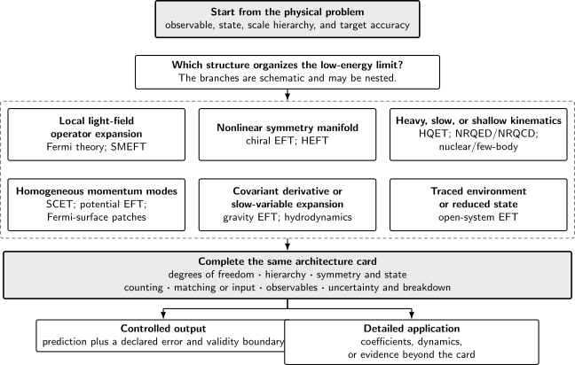
An EFT name is not a construction. Starting from the observable, state, scale hierarchy, and target accuracy, identify the dominant low-energy organizing structure, then declare degrees of freedom, symmetry and state, counting, matching or input, observables, uncertainty, and breakdown. Branches may be nested; the diagram is schematic and not to scale.
First application: a bounded Gaussian kernel
Section titled “First application: a bounded Gaussian kernel”Consider real histories on a finite interval , with and square-integrable and bounded by . The following is a supplied model, not the result of an environmental derivation:
with
where , , and ; the coefficients carry whatever units the chosen requires. The stationary kernels have memory time and are bounded on the finite domain.
| Kernel feature | Check | Interpretation |
|---|---|---|
| No term independent of | Coincident histories have influence factor one; reduced normalization is not lost | |
| Real term | Odd under and is real | Retarded response, including conservative renormalization and dissipation |
| Imaginary term | Even under and is real symmetric | Decoherence and Gaussian fluctuations |
| Step function in | for | The response is causal |
| Exponential tails | Both kernels decay on | Dynamics has finite memory and is not exactly local in time |
Hermiticity follows directly:
For the noise check, extend the stationary kernel to the real line or consider times far from the finite-interval boundaries. Its Fourier transform is
Therefore, for every real test history,
and . Equivalently, the imaginary term can be represented by averaging over a real Gaussian force with covariance . This verifies a well-defined noise kernel. It does not by itself prove that the full model comes from a positive microscopic state or defines a completely positive map for arbitrary parameters; those are stronger matching conditions.
The response and noise roles are distinct. Causality constrains the support of , positivity constrains the quadratic form defined by , and a thermal state would impose an additional fluctuation–dissipation relation between their frequency-dependent parts. No thermal relation has been assumed in this supplied model.
Testing the local-memory approximation
Section titled “Testing the local-memory approximation”For subsystem frequencies and times satisfying , the kernels admit a moment expansion. With the Fourier convention used above,
In time, the first response term is a local conservative shift and should be absorbed into a matched system parameter. The next term is local friction. The noise kernel approaches , with colored-noise corrections beginning at two additional derivatives. Initial-slip terms proportional to remain near the preparation time and are excluded by the stated late-time domain.
This is a controlled local-kernel approximation when
and when the histories being probed have no appreciable spectral support near . The first omitted response moment and noise moment provide separate truncation estimates. A sharp pulse, long environmental tail, near resonance, or leading initial correlation invalidates this expansion even if the coupling is numerically small.
White noise and a local friction term still do not automatically imply Lindblad evolution. They describe a local approximation to two kernels; complete positivity is a property of the entire reduced map.
A Lindblad limit needs stronger hypotheses
Section titled “A Lindblad limit needs stronger hypotheses”For a time-homogeneous, completely positive, trace-preserving Markov semigroup on a finite-dimensional subsystem—or on a field-theory operator domain where the generator is well defined—the generator has the Gorini–Kossakowski–Sudarshan–Lindblad form
The anticommutator and jump pieces cancel under the trace. Positivity of the Kossakowski matrix allows it to be diagonalized into nonnegative rates and Lindblad operators. This is the structural theorem under its semigroup hypotheses Gorini, Kossakowski, and Sudarshan 1976, pp. 821–825 and Lindblad 1976, pp. 119–130.
In the standard weak-coupling microscopic derivation, obtaining this limit ordinarily needs more than :
- environmental correlations decay on a time much shorter than subsystem evolution;
- the coupling is weak enough that the environment remains near its reference state;
- initial system–environment correlations are absent, parametrically suppressed, or included in a controlled preparation term;
- a coarse-graining interval exists with ;
- nonsecular frequency mixing can be dropped or otherwise treated without producing negative rates; and
- the resulting coefficient matrix is positive semidefinite over the retained operator basis.
A time-local master equation can fail the last condition, and a non-Markovian map can remain completely positive without being CP-divisible. “Local,” “Markovian,” and “Lindblad” are therefore not synonyms.
A simple EFT loss channel illustrates the trace constraint. If a retained nonrelativistic field disappears into energetic products that never return, take . Then
Keeping only the anti-Hermitian Hamiltonian would decrease . The jump term restores unit trace and transfers probability between retained particle-number sectors. Braaten, Hammer, and Lepage derive precisely this structure for deeply inelastic reaction products and show that the positive local rate matrix follows from the optical theorem Braaten, Hammer, and Lepage 2016, § II.B, pp. 3–4, Open PDF.
Failure boundaries and next applications
Section titled “Failure boundaries and next applications”The Gaussian example is intentionally bounded. It has one coordinate, stationary quadratic kernels, finite exponential memory, no displayed initial-correlation term, and no proof of a microscopic thermal or quantum uncertainty relation. Non-Gaussian noise, strong coupling, algebraic memory tails, driven environments, field-theory renormalization of influence kernels, and time-dependent subsystem splits require additional analysis.
The consistency workflow is:
- declare the subsystem, environment, state, observables, and time interval;
- verify coincident-history normalization, Hermiticity, causality, and noise-kernel positivity;
- identify the independent coupling, derivative, noise, and memory expansions;
- test the local approximation against the actual kernel moments and preparation time;
- claim a Lindblad limit only after establishing the Markov, coarse-graining, and positive-rate conditions; and
- attach an error estimate and state the validity boundary.
Deriving influence functionals by a microscopic trace, treating memory and nonlinear noise, and developing open-QFT applications continue in System–Environment Splits and Influence Functionals.
Common pitfalls
Section titled “Common pitfalls”Calling a partial trace Markovian. The exact reduced state generally remembers earlier environmental correlations. A local equation requires a correlation-time and coarse-graining hierarchy.
Using a non-Hermitian Hamiltonian alone. It describes probability leaving a sector but does not preserve the trace of the reduced density matrix. Jump terms are required when the lost probability remains part of the normalized subsystem description.
Equating a positive noise kernel with complete positivity. makes the Gaussian noise integral well defined. Complete positivity constrains the full map and can impose additional response–noise inequalities.
Calling every time-local equation Lindblad. A time-local generator with a non-positive rate matrix need not generate completely positive divisible evolution. State the theorem’s semigroup and domain assumptions.
Taking white noise before checking the spectrum. The expansion fails for pulses, resonances, or long memory. Estimate the first omitted moment and exclude the preparation-time boundary layer.
Imposing thermal fluctuation–dissipation without a thermal state. Hermiticity, normalization, and causality are more general than KMS. A thermal relation needs a thermal environmental state and its own frequency domain.
Equating open-system EFT with hydrodynamics. Conserved slow variables select hydrodynamics; a partial trace selects an open system. The two can nest, but neither criterion implies the other.
References
Section titled “References”-
Braaten, Eric, H.-W. Hammer, and G. Peter Lepage. 2016. “Open Effective Field Theories from Deeply Inelastic Reactions.” Physical Review D 94: 056006. DOI. Open PDF.
-
Feynman, Richard P., and Frank L. Vernon Jr. 1963. “The Theory of a General Quantum System Interacting with a Linear Dissipative System.” Annals of Physics 24: 118–173. DOI.
-
Gorini, Vittorio, Andrzej Kossakowski, and E. C. G. Sudarshan. 1976. “Completely Positive Dynamical Semigroups of N-Level Systems.” Journal of Mathematical Physics 17: 821–825. DOI.
-
Lindblad, Göran. 1976. “On the Generators of Quantum Dynamical Semigroups.” Communications in Mathematical Physics 48: 119–130. DOI.
Original QFT.org content:CC BY 4.0, unless an item supplies different terms. Third-party material retains its own terms.