

Ultraviolet Sensitivity and the Renormalization Problem
Short-distance singularities require new parameters because products of quantum fields at coincident points are not fixed by their separated-point behavior. Predictivity survives because the ultraviolet ambiguity is local: at any declared perturbative and EFT order, it can modify only a controlled set of local operators. Renormalization conditions fix the corresponding coefficients from the same number of inputs; every remaining quantity is a prediction, up to the stated truncation error.
This page separates four objects that must not be conflated: a regulator that makes intermediate expressions meaningful, bare parameters that depend on that regulated description, renormalized parameters defined by finite conditions, and non-input observables that should become regulator independent. A one-loop scalar two-point integral will show exactly where regulator dependence ends and invariant momentum dependence begins.
Required background. Coincident Products and Contact Terms supplies the distributional reason a new local extension is needed at coincidence.
Helpful background. Regulated Bosonic Field Integrals clarifies what a regulated measure defines, while Products, Scaling Degree, and Extensions of Singular Distributions gives a more precise mathematical language for the finite local ambiguity.
Ultraviolet sensitivity is sensitivity to unresolved local structure
Section titled “Ultraviolet sensitivity is sensitivity to unresolved local structure”A local interaction asks us to multiply fields at the same spacetime point. Even a free two-point function is singular as its arguments coincide, so perturbative products of propagators can fail to define distributions on those coincidence sets. Momentum space expresses the same problem through contributions from arbitrarily large loop momentum.
A regulator introduces auxiliary data that makes the expression well defined. Examples include a momentum cutoff , continuation to , Pauli–Villars masses, a lattice spacing , or a smooth kernel. At this stage the regulated Green function
depends on a regulator and on bare parameters . Neither dependence is normally observable. The regulator tells us how the unresolved region was temporarily represented; the bare parameters must vary with that representation if finite physical inputs are to remain fixed.
The crucial property is locality. For a graph whose ultraviolet degree permits subtraction through order , the ambiguous part has the form of a polynomial in the external momenta,
subject to the field content and symmetries. Fourier transformation turns momentum polynomials into derivatives of delta functions supported at coincident points. They are therefore generated by local terms in the action. Nonpolynomial momentum dependence—threshold square roots, branch cuts, and logarithms of kinematic ratios—cannot be chosen freely as a counterterm; it contains long-distance or finite dynamical information.
This is why renormalization adds parameters without surrendering prediction. At fixed order, the allowed polynomial space is finite-dimensional. Its coefficients are fixed by an equal number of renormalization conditions. Collins develops this relation between divergent graphs, local counterterms, and renormalization prescriptions in a form that includes subdivergences rather than only primitive one-loop examples Collins 1984/2023, §§ 3.1.3–3.4 and 5.1–5.5, pp. 41–60 and 89–113.
Bare parameters, renormalized inputs, and predictions
Section titled “Bare parameters, renormalized inputs, and predictions”For a scalar field, a conventional reparametrization is
where is fixed by the engineering dimension of the chosen interaction. This equation is an identity inside the regulated calculation. It does not split a measured quantity into independently measurable “bare” and “counterterm” pieces.
The roles are different:
| Object | How it is chosen | May depend on | What checks it |
|---|---|---|---|
| Regulator | Convenient auxiliary definition | cutoff shape, continuation, lattice, regulator masses | Removal or controlled-extrapolation limit |
| Bare data | Adjusted so finite input conditions hold | regulator and its removal trajectory | Reproduces the regulated action; not compared directly across regulators |
| Counterterms and | Cancel allowed local UV terms and implement finite conditions | regulator, subtraction scheme, scale , perturbative order | Locality, symmetry identity, and order bookkeeping |
| Renormalized parameters | Coordinates defined by stated renormalization conditions | scheme and, generally, | Recover the chosen input data |
| Non-input prediction | Calculated after inputs are fixed | physical kinematics and masses; residual scheme dependence beyond truncation | Agreement between matched regulators or schemes and with observation |
Follow the dashed paths from common finite inputs to calculations A and B. These are independent regulator choices, not successive steps; their solid output paths compare a non-input quantity at the same kinematics and order.
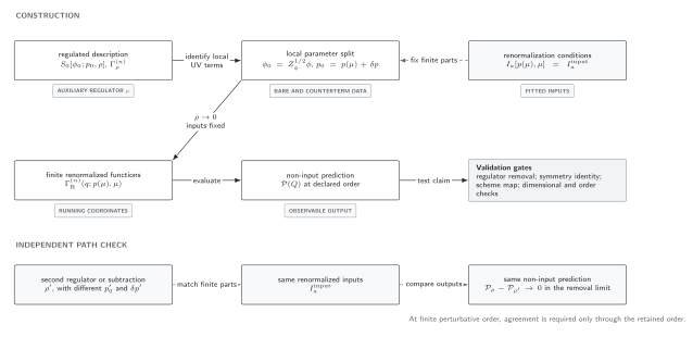
Two regulators, one set of finite input and normalization conditions. Each branch tunes its own bare parameters and allowed local counterterms. Restoring the same identities and translating finite schemes makes the outputs agree through the retained order Collins 1984/2023, § 7.10, pp. 206–208. Vanishing regulator artifacts and uncomputed perturbative terms remain distinct. This schematic map is not a nonperturbative continuum construction.
Two immediate consequences are easy to miss.
First, holding fixed while changing or removing the regulator generally changes the physical theory. The correct comparison holds the chosen renormalized inputs fixed and lets follow the required trajectory. Second, selecting a regulator cannot define the continuum theory by itself. With the same cutoff one may impose different finite mass or coupling conditions and obtain physically different predictions; the missing information is the renormalized input, not a better ultraviolet damping function.
One-loop two-point comparison
Section titled “One-loop two-point comparison”Consider the Euclidean scalar bubble
It occurs, with theory-dependent coupling and symmetry factors, in a one-loop scalar self-energy. We suppress those overall factors to isolate the ultraviolet structure. The mass and Euclidean momentum keep the example infrared safe; analytic continuation and the physical cut are separate questions.
Dimensional regulator
Section titled “Dimensional regulator”With and the scale factor ,
where
The pole is independent of : it is local and can be absorbed into the permitted two-point counterterm. The Feynman-parameter integral contains the finite momentum dependence.
Momentum cutoff
Section titled “Momentum cutoff”For a rotationally invariant hard cutoff, the large- form can be organized as
Here is an arbitrary reference used only to make logarithms dimensionless, and depends on the precise cutoff definition and momentum routing convention. The divergent logarithm and differ from the dimensional result, but they are again independent of external momentum. The nonlocal dependence agrees.
Match the same finite condition
Section titled “Match the same finite condition”Define a momentum-subtracted quantity by fixing the two-point function at a Euclidean reference momentum :
For dimensional regularization, means after subtraction; for the cutoff it means . Both give
The pole, cutoff logarithm, and regulator-dependent constant have disappeared. What remains is the momentum dependence relative to the chosen input point. In a complete two-point function, the superficial degree determines whether mass, field-strength, or higher-derivative conditions are required; this logarithmic example needs only the constant subtraction shown.
The derivative provides a sharp check:
It is finite, regulator independent, and has mass dimension . Differentiation has removed the degree-zero local ambiguity but not the dynamical momentum dependence. This simple operation anticipates the general statement: sufficiently many external-momentum derivatives make a superficially divergent graph convergent, leaving only an integration polynomial to be fixed locally.
Why the theory remains predictive
Section titled “Why the theory remains predictive”Suppose the action contains independent local coefficients that can contribute through a specified order. Fixing independent renormalization conditions determines those coefficients. A calculation of an st quantity is then constrained. Changing a regulator or subtraction prescription changes the coordinates used in that calculation, not the number of independent inputs.
In a power-counting-renormalizable theory, the same finite set of action monomials suffices to all perturbative orders, although their coefficients are corrected order by order. In an EFT, infinitely many local operators are allowed in principle, but only finitely many contribute at any fixed order in the declared expansion. Predictivity therefore comes from an ordering principle and a truncation estimate, not from forbidding every interaction of high canonical dimension.
The logic can be expressed as a count:
This is schematic, because symmetries can relate inputs and observables and because redundant parameters must first be removed. Its point is conceptual: a counterterm coefficient is not a new adjustable number every time a graph is drawn. One coefficient renormalizes every occurrence of the same local operator, and symmetry identities can tie several counterterms together.
Regulator independence is an operational claim
Section titled “Regulator independence is an operational claim”“The answer is regulator independent” should be supported by a reproducible comparison, not assumed from notation. A useful record contains:
- the regulated object and external kinematic regime;
- the regulator and its removal variable;
- the complete local counterterm space at the retained order;
- the renormalization conditions and which quantities are treated as inputs;
- the bare-parameter trajectory needed to preserve those inputs;
- the limit or extrapolation of at least one non-input quantity;
- symmetry and dimensional checks; and
- the expected perturbative or cutoff-suppressed remainder.
At finite perturbative order, two schemes need not give numerically identical intermediate parameters or exactly identical truncated predictions. After applying the finite parameter map, their difference should begin at the first omitted order. Residual dependence is then a useful diagnostic, but it is not automatically a probability distribution for the error.
The claim also has limits. A regulator may break a symmetry, requiring allowed restoration counterterms or revealing an anomaly. A massless example can mix ultraviolet and infrared singularities, so a zero scaleless integral cannot be used as the ultraviolet diagnosis. A cutoff EFT may deliberately retain a finite cutoff below its breakdown scale; the validation target is cutoff stability within the EFT error, not necessarily an infinite-cutoff limit. And perturbative removal order by order is not a nonperturbative existence proof for the continuum theory.
Common pitfalls
Section titled “Common pitfalls”Comparing bare parameters. Bare masses and couplings in two regulators are not expected to agree. Match the same finite renormalized inputs, follow each bare trajectory, and compare a non-input prediction.
Calling every divergent term unphysical. The divergent coefficient is auxiliary, but the local operator it multiplies represents genuine short-distance information that must be fixed. Removing the divergence does not determine its finite coefficient.
Subtracting nonlocal momentum dependence. A counterterm such as is nonlocal and would erase dynamical information rather than choose a local extension. The subtraction ambiguity is polynomial to the degree allowed by power counting.
Holding the wrong quantity fixed. Taking at fixed bare mass generally does not preserve the physical pole or a chosen Euclidean mass condition. State the renormalized inputs before taking the limit.
Inferring ultraviolet completion. Order-by-order renormalizability establishes a perturbative construction around the declared regime. It does not by itself prove that an interacting continuum theory exists at arbitrarily high energy.
Exercises
Section titled “Exercises”1. Local versus nonlocal. In the large-cutoff expansion
which terms can be changed by local two-point counterterms?
Solution
The term is momentum independent and local. The coefficient multiplying is also local because its external-momentum dependence is polynomial; it is absorbed by a kinetic counterterm. The term is nonpolynomial and must remain, up to local finite polynomials fixed by the renormalization conditions.
2. Wrong fixed quantity. Two cutoff calculations use the same numerical bare mass but different cutoff shapes. Must their renormalized pole masses agree?
Solution
No. The relation between bare and renormalized mass depends on the regulator. To compare the same theory, impose the same finite mass condition in both calculations and adjust the two bare masses accordingly. A separate non-input observable should then agree in the removal limit, within the retained-order remainder.
3. Bubble subtraction. Verify directly that and that has mass dimension .
Solution
At the logarithm’s numerator and denominator coincide for every , so the integral vanishes. Differentiation produces a denominator of mass dimension two and a dimensionless numerator and measure, hence dimension . Both checks are independent of the regulator-specific local constant.
What this page establishes
Section titled “What this page establishes”The renormalization problem is not the appearance of a large symbol such as or . It is the need to define local short-distance data consistently with symmetry and then demonstrate that non-input predictions do not depend on the auxiliary definition. The one-loop comparison made the separation explicit:
Changing the regulator changes the first term and the bare trajectory. Changing a renormalization scheme changes the finite coordinate assigned to the second. Neither may alter the third after the same inputs are matched, except by terms beyond the declared approximation.
Continue to Power Counting of Divergences and Perturbative Renormalizability to determine which local structures can occur before evaluating a graph. Use QFT Regulator Families and Their Tradeoffs when the next decision is which properties a regulator should preserve. The chapter overview gives the full route from ultraviolet diagnosis to a regulator-removal test.
References
Section titled “References”- Collins, John C. 1984; open-access reissue 2023. Renormalization: An Introduction to Renormalization, the Renormalization Group and the Operator-Product Expansion. Cambridge Monographs on Mathematical Physics. Cambridge University Press. DOI and Open PDF.
Original QFT.org content:CC BY 4.0, unless an item supplies different terms. Third-party material retains its own terms.