Fixed Points and Linearized RG Flow

A renormalization-group fixed point is a scale-invariant point in the space of dimensionless actions or couplings. Linearizing the RG flow there turns an otherwise nonlinear problem into a spectral one: the eigenoperators of the stability operator are the scaling perturbations, and their eigenvalues decide which departures grow or decay. This page derives that statement, works a nontrivial two-coupling example, and marks the boundary beyond which local linear data no longer determine the flow.

Required background. Wilsonian Coarse Graining and Theory Space supplies the interpretation of RG evolution as coarse graining followed by rescaling. Helpful background. Normal Forms, Spectra, and Projectors reviews eigenvectors and Jordan form, while Multiple Couplings and Coupled RG Flows develops beta functions as a vector field.

Fixed points in dimensionless theory space

Let $g^i(k)$ denote dimensionless coordinates on a finite-dimensional approximation to theory space. The same construction applies to the full action, with indices replaced by continuous labels and the stability matrix by a linear operator. Throughout this chapter,

$$t\equiv\ln\frac{k}{\Lambda_{\mathrm{UV}}}, \qquad \partial_t g^i=\beta^i(g).$$

Lowering the coarse-graining scale $k$ moves toward the infrared and decreases $t$. This orientation must be declared before words such as “attractive” are assigned: reversing RG time reverses attraction, although it does not change the operator classification.

A fixed point $g_\star$ satisfies

$$\beta^i(g_\star)=0.$$

The word “dimensionless” is essential. A mass parameter can run simply because it carries units; its dimensionless counterpart $m^2/k^2$ is the coordinate whose constancy signals scale invariance. Likewise, a fixed action means that all rescalings needed to compare successive coarse-grained theories have already been made. The resulting theory may possess anomalous field dimensions, so scale invariance does not mean that every field retains its engineering dimension.

For finitely many couplings, a fixed point is a common zero of their beta functions. In exact Wilsonian language it is a functional solution

$$\partial_t S_k[\phi]=\mathcal F[S_k]=0$$

after fields, coordinates, and the action have been rendered dimensionless. A zero found only after projecting $\mathcal F$ onto a truncation is therefore a candidate fixed point of that approximation. Its persistence under enlargement of the ansatz is an evidence question, not part of the definition.

The stability operator and scaling perturbations

Write $g^i=g_\star^i+\delta g^i$. Taylor expansion gives

$$\partial_t\delta g^i = B^i{}_j\,\delta g^j+O(\delta g^2), \qquad B^i{}_j \equiv \left. \frac{\partial\beta^i}{\partial g^j} \right|_{g_\star}.$$

We define right eigenvectors $V_I$ and critical exponents $\theta_I$ by

$$B V_I=-\theta_I V_I.$$

If $B$ is diagonalizable and the eigenvectors span the perturbations under consideration, then

$$\delta g(t) = \sum_I C_I e^{-\theta_I(t-t_0)}V_I.$$

For motion from $t_0$ toward the infrared, $t-t_0<0$. Consequently a component with $\theta_I>0$ grows, one with $\theta_I<0$ decays, and linear order says nothing when $\theta_I=0$.

Critical exponent	As $k$ decreases	As $k$ increases	Linear name
$\theta_I>0$	grows away from the fixed point	decays toward the fixed point	relevant
$\theta_I<0$	decays toward the fixed point	grows away from the fixed point	irrelevant
$\theta_I=0$	unresolved at linear order	unresolved at linear order	marginal

Thus “relevant” and “UV-attractive” describe the same direction viewed in opposite limits under this convention. It is clearer to reserve relevant, marginal, and irrelevant for the eigenoperator, and to state the UV or IR orientation separately.

The least-negative irrelevant exponent is conventionally written $\theta_{\mathrm{irr}}=-\omega$ with $\omega>0$; it controls the leading generic correction to asymptotic scaling when the corresponding amplitude is nonzero. Wegner develops this expansion in irrelevant scaling fields in Wegner 1972, pp. 4529–4534.

In action language, a perturbation takes the form

$$S=S_\star+\sum_I c_I\!\int\! d^dx\,\mathcal O_I(x).$$

After operator mixing has been diagonalized, the coupling to a scalar eigenoperator of scaling dimension $\Delta_I$ has

$$\theta_I=d-\Delta_I.$$

This relation includes anomalous dimensions: if $\Delta_I=\Delta_I^{\mathrm{eng}}+\gamma_I^\star$, then $\gamma_I^\star$ is evaluated at the fixed point and shifts the RG eigenvalue away from canonical power counting. Operators that vanish by field redefinitions or equations of motion generate redundant directions; their eigenvalues can appear in a coordinate description without representing independent physical deformations. Physical tuning counts require quotienting those directions.

Wilson and Kogut derive the connection among fixed points, eigenoperators, and scaling fields in Wilson and Kogut 1974, §§ 11–12, pp. 152–176.

Worked example: a nontrivial two-coupling fixed point

Consider two dimensionless couplings $g_1,g_2$ and shift the candidate fixed point to the origin,

$$x\equiv g_1-1, \qquad y\equiv g_2-1.$$

Take the polynomial flow

$$\beta_x=-2x+y+xy, \qquad \beta_y=y+x^2.$$

This is a deliberately transparent model of a coupled RG vector field, not the beta function of a particular microscopic Lagrangian. It nevertheless contains the local structures that recur in QFT calculations.

The fixed-point equations can be solved without numerical root finding. From $\beta_y=0$,

$$y=-x^2.$$

Substitution into $\beta_x=0$ gives

$$0=-x\left(x^2+x+2\right).$$

The quadratic factor has discriminant $1-8=-7$, so the only real solution is $x=y=0$. In the original coordinates the fixed point is therefore nontrivial:

$$(g_{1\star},g_{2\star})=(1,1).$$

The stability matrix is

$$B = \left. \begin{pmatrix} -2+y & 1+x\\ 2x & 1 \end{pmatrix} \right|_{x=y=0} = \begin{pmatrix} -2 & 1\\ 0 & 1 \end{pmatrix}.$$

Its eigenpairs, expressed using $B V=-\theta V$, are

$$\begin{aligned} \theta_{\mathrm{rel}}&=2, &V_{\mathrm{rel}}&=\begin{pmatrix}1\\0\end{pmatrix},\\ \theta_{\mathrm{irr}}&=-1, &V_{\mathrm{irr}}&=\begin{pmatrix}1\\3\end{pmatrix}. \end{aligned}$$

Hence the linearized solution is

$$\begin{pmatrix}x(t)\\y(t)\end{pmatrix} = C_{\mathrm{rel}}e^{-2(t-t_0)} \begin{pmatrix}1\\0\end{pmatrix} + C_{\mathrm{irr}}e^{t-t_0} \begin{pmatrix}1\\3\end{pmatrix}.$$

As $k$ decreases, the first term grows and the second decays. A trajectory reaches the fixed point in the infrared only if its relevant coefficient is tuned to zero. At linear order the critical surface is therefore tangent to $V_{\mathrm{irr}}$ and has codimension one.

The corresponding scaling coordinates are

$$s_{\mathrm{irr}}=\frac{y}{3}, \qquad s_{\mathrm{rel}}=x-\frac{y}{3},$$

so that $x=s_{\mathrm{rel}}+s_{\mathrm{irr}}$ and $y=3s_{\mathrm{irr}}$. Keeping the nonlinear terms reveals why the tangent-space answer is not the whole critical surface:

$$\begin{aligned} \partial_t s_{\mathrm{rel}} &=-2s_{\mathrm{rel}} -\frac13s_{\mathrm{rel}}^2 +\frac73s_{\mathrm{rel}}s_{\mathrm{irr}} +\frac83s_{\mathrm{irr}}^2,\\ \partial_t s_{\mathrm{irr}} &=s_{\mathrm{irr}} +\frac13 \left(s_{\mathrm{rel}}+s_{\mathrm{irr}}\right)^2. \end{aligned}$$

Even when $s_{\mathrm{rel}}=0$ at one point, the term $8s_{\mathrm{irr}}^2/3$ regenerates it. The exact local stable manifold is curved; the eigenvector supplies only its tangent at the fixed point. An interactive calculation can compare this linear approximation with the nonlinear trajectories.

The figure below summarizes what to inspect: the tangent directions in panel (a), their competing exponential magnitudes in panel (b), and a standard QFT realization together with a limitation of naive scaling in panel (c).

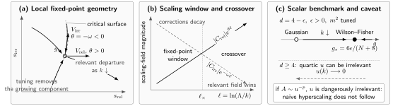
A fixed point organizes local flow, not every global trajectory. Panel (a) shows the critical surface tangent to the irrelevant eigendirection and the relevant departure under infrared flow. Panel (b) compares $e^{\theta\ell}$ growth with $e^{-\omega\ell}$ corrections for $\ell=\ln(\Lambda/k)$. Panel (c) shows the tuned one-loop $O(N)$ scalar trajectory from the Gaussian point to $g_\star=6\epsilon/(N+8)$ and the dangerously irrelevant-coupling exception to naive hyperscaling. The diagram is schematic and not to scale.

What survives a change of coupling coordinates

Let $g'^a=f^a(g)$ be an analytic, locally invertible reparametrization, with Jacobian $J^a{}_i=\partial f^a/\partial g^i$. The transformed beta function is a vector,

$$\beta'^a(g')=J^a{}_i(g)\,\beta^i(g).$$

Differentiating produces a term proportional to $\partial J\,\beta$. That term vanishes at a fixed point, leaving

$$B'=J_\star B J_\star^{-1}.$$

The exact stability matrices are related by similarity. Their eigenvalues, algebraic multiplicities, and Jordan structure are therefore coordinate invariant, while the numerical coordinates $g_\star^i$ and components of each eigenvector are not.

For example, applying $u=x+y$, $v=y$ to the worked flow gives

$$J=\begin{pmatrix}1&1\\0&1\end{pmatrix}, \qquad B'=\begin{pmatrix}-2&4\\0&1\end{pmatrix}.$$

The entries change, but the critical exponents remain $2$ and $-1$. This invariance assumes an exact fixed point and an invertible Jacobian. Singular transformations can add or remove apparent directions; scale-dependent redefinitions require extra terms; and two finite truncations need not be related by an exact similarity transformation. Fixed-point coordinates are consequently poor scheme-invariance tests, whereas stable physical exponents are meaningful comparison targets.

Field redefinitions sharpen the same warning. A tangent generated solely by changing variables in the functional integral is redundant. One should identify observables or nonredundant operator classes before interpreting every eigenvalue of a projected matrix as a new measurable exponent. Wegner’s invariance analysis makes this distinction precise in Wegner 1974, pp. 2098–2105.

Continuous flow, blocking steps, and anomalous scaling

A discrete Wilsonian transformation that lowers the cutoff by a factor $b>1$ sends $t$ to $t-\ln b$. The continuous solution therefore implies

$$\delta g_I(t-\ln b) =b^{\theta_I}\delta g_I(t).$$

Thus the eigenvalue of the linearized blocking map is $b^{\theta_I}$. This is the bridge between notation using a scaling power $y_I$ and notation using a continuous critical exponent $\theta_I$: with the same direction of blocking, $y_I=\theta_I$.

The rescaling part of the RG step also fixes the field dimension. For a scalar field,

$$\Delta_\phi=\frac{d-2+\eta}{2},$$

where $\eta$ is the fixed-point anomalous dimension. Composite eigenoperators generally mix, so their anomalous dimensions are eigenvalues of a mixing problem rather than derivatives of isolated beta functions. A consistent stability analysis therefore requires all couplings that mix at the target accuracy, including wave-function normalization when $\eta$ matters.

The celebrated Wilson–Fisher construction is an example: below four dimensions the quartic scalar interaction acquires a nonzero fixed-point coordinate of order $\epsilon$, and linearization produces noncanonical scaling exponents. The original controlled expansion is given in Wilson and Fisher 1972, pp. 240–243. The dedicated Gaussian and Wilson–Fisher Fixed Points page works that QFT calculation in the normalization used by the figure.

When eigenvalues are not enough

The compact exponential solution rests on assumptions that should be checked rather than silently inherited.

Marginal directions. If $\theta=0$, the first nonzero nonlinear term decides the flow. For a scaling coordinate $u$ with $\partial_tu=a u^2+O(u^3)$, the sign of $a$ and the side from which $u$ approaches zero determine marginal relevance or irrelevance. A continuous line of fixed points instead has a genuine tangent zero mode after redundancies are removed.

Jordan blocks. If $B$ is not diagonalizable, generalized eigenvectors produce powers of $t-t_0$ multiplying the exponential. A repeated eigenvalue alone does not establish a Jordan block; its geometric multiplicity must also be checked.

Complex eigenvalues. A conjugate pair $\theta=\theta_R\pm i\theta_I$ gives spiraling linear trajectories. The sign of $\theta_R$ controls radial growth or decay, while $\theta_I$ sets rotation in logarithmic scale. Whether such behavior is compatible with reflection positivity, unitarity, or other properties depends on the theory and cannot be inferred from the matrix alone.

Non-normal flow. Even with a complete spectrum, nonorthogonal eigenvectors can cause transient amplification before the asymptotic exponent dominates. Left eigenvectors, not Euclidean dot products with right eigenvectors, extract the coefficients $C_I$ in a general basis.

Finite domain. Linearization is trustworthy only while $\lVert\delta g\rVert$ is small enough that the omitted nonlinear terms remain subleading. A relevant perturbation inevitably exits that neighborhood under infrared evolution. The resulting departure scale is physical crossover data, but predicting what happens afterward requires the full beta functions.

Global alternatives. Fixed-point collisions, walking regions, limit cycles, singular boundaries, and disconnected basins are global properties. A local stability matrix neither discovers them nor rules them out. It also does not prove that a candidate trajectory defines a unitary, local continuum QFT.

The next page, Relevant, Marginal, and Irrelevant Directions, turns these qualifications into an operator-by-operator classification.

A compact fixed-point check

Before interpreting a computed spectrum, verify the following in order:

1. All couplings and fields used in the fixed-point equation are dimensionless.
2. The direction of RG time and the sign convention in $B V=-\theta V$ are explicit.
3. The beta functions vanish to the stated analytic or numerical tolerance.
4. The stability matrix includes the mixing needed at the claimed accuracy.
5. Eigenvectors, degeneracies, complex pairs, and Jordan structure have been checked.
6. Redundant directions have been identified before counting physical tunings.
7. Coordinate, scheme, regulator, and truncation variations are separated from universal claims.
8. Conclusions are restricted to the neighborhood where nonlinear remainders are controlled.

This sequence prevents two common category errors: treating a beta-function zero as a complete theory, and treating raw coupling coordinates as universal observables.

Exercises

1. Check the coordinate transformation

For $u=x+y$ and $v=y$, derive $B'=J B J^{-1}$ for the worked example and find its eigenvectors.

Solution

Here

$$J=\begin{pmatrix}1&1\\0&1\end{pmatrix}, \qquad J^{-1}=\begin{pmatrix}1&-1\\0&1\end{pmatrix}.$$

Direct multiplication gives

$$B'=J B J^{-1} =\begin{pmatrix}-2&4\\0&1\end{pmatrix}.$$

For eigenvalue $-2$, one may take $V'_{\mathrm{rel}}=(1,0)^T=J V_{\mathrm{rel}}$. For eigenvalue $1$, one may take $V'_{\mathrm{irr}}=(4,3)^T=J V_{\mathrm{irr}}$. The components change exactly as tangent vectors should, while $\theta_{\mathrm{rel}}=2$ and $\theta_{\mathrm{irr}}=-1$ do not.

2. Solve a Jordan-block flow

Let

$$B=\begin{pmatrix}-\theta&1\\0&-\theta\end{pmatrix}.$$

Solve $\partial_t\delta g=B\delta g$ with initial data $(x_0,y_0)$ at $t=t_0$.

Solution

Writing $\tau=t-t_0$, the second equation gives $y(\tau)=e^{-\theta\tau}y_0$. An integrating factor in the first equation then gives

$$x(\tau)=e^{-\theta\tau}(x_0+\tau y_0).$$

Therefore

$$\delta g(\tau) =e^{-\theta\tau} \begin{pmatrix}x_0+\tau y_0\\y_0\end{pmatrix}.$$

The polynomial factor $\tau$ is the signature missed by a list containing only the repeated eigenvalue.

3. Recover Gaussian power counting

At a Gaussian fixed point, a scalar operator $\mathcal O$ has engineering dimension $\Delta_{\mathcal O}$. Show how its integrated coupling is classified.

Solution

The action perturbation $c\int d^dx\,\mathcal O$ is dimensionless, so $c$ has mass dimension $d-\Delta_{\mathcal O}$. With no anomalous contribution at the Gaussian point,

$$\theta=d-\Delta_{\mathcal O}.$$

The deformation is relevant if $\Delta_{\mathcal O}<d$, marginal if $\Delta_{\mathcal O}=d$, and irrelevant if $\Delta_{\mathcal O}>d$. Interactions can shift this result because the fixed-point operator dimension is then $\Delta_{\mathcal O}^{\mathrm{eng}}+\gamma_{\mathcal O}^\star$.

References

• Wegner, Franz J. “Corrections to Scaling Laws.” Physical Review B 5 (1972): 4529–4536. DOI.
• Wegner, Franz J. “Some Invariance Properties of the Renormalization Group.” Journal of Physics C: Solid State Physics 7 (1974): 2098–2108. DOI.
• Wilson, Kenneth G., and Michael E. Fisher. “Critical Exponents in 3.99 Dimensions.” Physical Review Letters 28 (1972): 240–243. DOI.
• Wilson, Kenneth G., and John Kogut. “The Renormalization Group and the $\epsilon$ Expansion.” Physics Reports 12 (1974): 75–200. DOI.