Critical Surfaces, Crossover, and Corrections to Scaling

A critical surface is the set of actions whose RG trajectories approach a fixed point in a specified limit. Its tangent space is determined by stability eigenvectors, but its curvature, basin, and crossover trajectories are nonlinear data. This page constructs a local critical surface, counts tunings in the IR and UV orientations, derives crossover variables and scales, and shows how irrelevant perturbations produce finite-size and finite-cutoff corrections.

Required background. Relevant, Marginal, and Irrelevant Directions supplies the convention $B V_I=-\theta_I V_I$ and the physical distinction among relevant, irrelevant, marginal, dangerous, and redundant perturbations.

Critical manifolds in infrared RG time

It is convenient to follow coarse graining with

$$\ell\equiv\ln\frac{\Lambda}{k},$$

so $\ell$ increases toward the infrared. In local scaling coordinates $s_I$ around a fixed point,

$$\frac{d s_I}{d\ell} =\theta_I s_I+O(s^2).$$

A relevant coordinate with $\theta_I>0$ grows, while an irrelevant coordinate with $\theta_I<0$ decays. If no eigenvalue has zero real part and the beta-function vector field is sufficiently smooth, local stable- and unstable-manifold results give invariant manifolds tangent to the corresponding eigenspaces.

For an infrared fixed point, the local critical surface $\mathcal S_{\mathrm{IR}}$ is tangent to the irrelevant eigenspace. If there are $n_{\mathrm{rel}}$ independent physical relevant directions, then

$$\operatorname{codim}\mathcal S_{\mathrm{IR}} =n_{\mathrm{rel}}.$$

Reaching the fixed point requires one tuning for each relevant component. Redundant directions are removed before this count. Marginal directions require a center-manifold or nonlinear analysis and are not assigned to either side merely from the zero eigenvalue.

Near a scalar critical point with one relevant temperature-like field, the bare mass must be adjusted to a critical value that depends on all other microscopic couplings:

$$m_0^2=m_{\mathrm c}^2(\lambda_0,c_{6,0},\ldots).$$

The graph of this function is the critical surface in those coordinates. Changing an irrelevant bare coupling generally shifts the nonuniversal value $m_{\mathrm c}^2$ even though its own scaling field decays and the asymptotic critical exponents remain unchanged.

Wilson and Kogut construct critical surfaces and their relevant departures in Wilson and Kogut 1974, §§ 11–12, pp. 159–176.

Constructing the curved surface in a two-coupling flow

Return to the two-coupling example written in its linear eigenvector coordinates,

$$r\equiv s_{\mathrm{rel}}, \qquad q\equiv s_{\mathrm{irr}}.$$

In the original RG time $t=\ln(k/\Lambda)$, its exact polynomial flow is

$$\begin{aligned} \partial_t r &=-2r-\frac13r^2+\frac73rq+\frac83q^2,\\ \partial_t q &=q+\frac13(r+q)^2. \end{aligned}$$

The linear critical surface is $r=0$, but it is not invariant: substituting $r=0$ gives $\partial_t r=8q^2/3$. Seek the nonlinear surface as a graph

$$r=h(q)=a q^2+b q^3+O(q^4).$$

Invariance requires the vector field to be tangent to the graph,

$$h'(q)\,\partial_tq =\left.\partial_t r\right|_{r=h(q)}.$$

Expanding both sides gives

$$\begin{aligned} h'(q)\,\partial_tq &=2a q^2+\left(\frac{2a}{3}+3b\right)q^3+O(q^4),\\ \left.\partial_t r\right|_{r=h(q)} &=\left(-2a+\frac83\right)q^2 +\left(-2b+\frac{7a}{3}\right)q^3 +O(q^4). \end{aligned}$$

Matching powers yields

$$a=\frac23, \qquad b=\frac29.$$

Thus

$$\boxed{ r=\frac23q^2+\frac29q^3+O(q^4) }$$

is the local infrared critical surface through cubic order. Its tangent is indeed the irrelevant eigendirection $r=0$, but a trajectory initialized on that tangent line rather than on the curved graph acquires a relevant component at order $q^2$.

In the original shifted coordinates $x=g_1-1$, $y=g_2-1$, where $q=y/3$ and $r=x-y/3$, the same result is

$$x =\frac{y}{3} +\frac{2y^2}{27} +\frac{2y^3}{243} +O(y^4).$$

This construction is local. Continuing the series does not by itself determine whether the surface folds, meets another fixed point, terminates at a singularity, or bounds a first-order region.

A scalar tuning, crossover, and correction calculation

Let $\tau$ be the tuned scalar mass scaling field, $h$ a second relevant deformation, and $u$ the leading ordinary irrelevant field. Their local infrared evolution is

$$\tau(\ell)=\tau_0e^{y_t\ell}, \qquad h(\ell)=h_0e^{y_h\ell}, \qquad u(\ell)=u_0e^{-\omega\ell},$$

with $y_t,y_h,\omega>0$. Tuning the mass means setting the nonlinear scaling coordinate $\tau_0$ to zero, not merely setting a convenient bare mass parameter to zero.

If $\tau_0=0$ but $h_0\neq0$, the second relevant field eventually becomes order one. Its departure scale follows from

$$|h_0|e^{y_h\ell_h}\sim1,$$

so

$$\ell_h\simeq\frac{1}{y_h}\ln\frac{1}{|h_0|}, \qquad k_h\simeq\Lambda |h_0|^{1/y_h}.$$

Above $k_h$ the trajectory can display approximate fixed-point scaling; below it the flow crosses over to behavior governed by the deformation. For a magnetic field at an Ising-like critical point, the sharp zero-field transition is rounded.

When both relevant fields are nonzero, choose the scale at which $|\tau|$ becomes order one. The invariant competition variable is

$$X = \frac{h}{|\tau|^{\phi}}, \qquad \phi=\frac{y_h}{y_t}=\nu y_h.$$

The exponent $\phi$ is a crossover exponent. The limits $X\ll1$, $X\sim1$, and $X\gg1$ select different portions of one scaling function; they are not three unrelated power laws.

At the same matching scale, the irrelevant argument is

$$u_0e^{-\omega\ell_\tau} =u_0|\tau|^{\omega/y_t} =u_0|\tau|^{\omega\nu}.$$

Provided the observable is regular as this argument tends to zero,

$$\mathcal O(\tau,h,u) = |\tau|^{-x_{\mathcal O}} \left[ F_0(X) +u_0|\tau|^{\omega\nu}F_1(X) +\cdots \right].$$

This single expression contains mass tuning, crossover under a separate relevant deformation, and the leading correction from an irrelevant perturbation. If $F_0$ or $F_1$ is singular as $u\to0$, the ordinary expansion fails and the variable is dangerously irrelevant.

Finite size, finite cutoff, and effective exponents

At criticality in a box of linear size $L$, choose the blocking factor $b=L/a$, where $a$ is a microscopic cutoff length. A dimensionless observable has the generic form

$$R(L) =R_\star +c_1L^{-\omega} +c_2L^{-\omega_2} +c_{\mathrm a}L^{-p} +\cdots,$$

after powers of $a$ have been absorbed into the coefficients. The $\omega_i$ terms come from irrelevant eigenoperators; $p$ can represent analytic, lattice-symmetry, or observable-specific corrections. A small fitted $c_1$ does not prove that the $\omega$ direction is absent—it may reflect an improved microscopic action or an accidental overlap zero.

With an ultraviolet cutoff $\Lambda$ and a running infrared scale $k$, the same leading irrelevant component behaves as

$$u(k)\sim u(\Lambda) \left(\frac{k}{\Lambda}\right)^{\omega}.$$

This is the residual finite-cutoff correction inside the fixed-point regime. A trustworthy continuum claim varies $\Lambda$, includes all allowed counterterms, and separates this power from ordinary perturbative truncation and numerical error.

Preasymptotic data are often summarized by an effective exponent. If

$$X(\tau)=A|\tau|^{-x} \left(1+a|\tau|^{\Delta}+\cdots\right),$$

define

$$x_{\mathrm{eff}}(\tau) \equiv -\frac{d\ln X}{d\ln|\tau|} =x- \frac{a\Delta|\tau|^{\Delta}} {1+a|\tau|^{\Delta}} +\cdots.$$

A drifting effective exponent can therefore be the expected approach to a fixed point, crossover away from it, or competition among several corrections. A plateau is persuasive only when the fit window also satisfies scale separation from the cutoff, finite volume, and the departure scale.

Wegner’s irrelevant-field expansion provides the systematic correction powers Wegner 1972, pp. 4529–4534. Riedel and Wegner show how competing relevant fields generate crossover exponents and effective critical behavior in Riedel and Wegner 1972, pp. 349–352.

Reading the local geometry

The shared figure keeps three statements separate. Panel (a) shows a critical surface only through its local tangent and a relevant departure; panel (b) shows why irrelevant corrections can decay before a mistuning drives crossover; panel (c) warns that a vanishing irrelevant coupling may still control an amplitude.

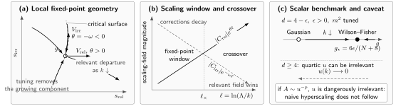
A fixed point organizes local flow, not every global trajectory. Panel (a) shows the critical surface tangent to the irrelevant eigendirection and the relevant departure under infrared flow. Panel (b) compares $e^{\theta\ell}$ growth with $e^{-\omega\ell}$ corrections for $\ell=\ln(\Lambda/k)$. Panel (c) shows the tuned one-loop $O(N)$ scalar trajectory from the Gaussian point to $g_\star=6\epsilon/(N+8)$ and the dangerously irrelevant-coupling exception to naive hyperscaling. The diagram is schematic and not to scale.

The Universality Classes and Scaling Functions page next explains which parts of $F_0(X)$ survive changes of microscopic realization.

Infrared and ultraviolet critical surfaces

The same phrase is used in two orientations, so the limiting direction must be attached to it.

Limit	Directions tangent to the local surface	Dimension or codimension statement	Physical interpretation
IR fixed point, $k\to0$	IR-attractive directions, $\theta<0$	codimension equals the number of physical relevant directions	relevant scaling fields must be tuned away to remain critical
UV fixed point, $k\to\infty$	UV-attractive directions, $\theta>0$	dimension equals the number of physical relevant directions	coordinates along the surface are free renormalized parameters locally

For a UV continuum limit, components with $\theta<0$ grow as $k\to\infty$ and must be fixed as functions of the coordinates on the UV critical surface. Saying that a theory has $n_{\mathrm{rel}}$ relevant directions therefore means that its local UV critical surface has dimension $n_{\mathrm{rel}}$, not that $n_{\mathrm{rel}}$ additional quantities must be tuned to zero. In an infinite truncation, finiteness of this physical dimension is the local predictivity criterion; it is not proof of global existence, unitarity, or the desired infrared endpoint.

Common pitfalls

Confusing a tangent plane with the critical surface. Eigenvectors determine the tangent at the fixed point. Quadratic terms can regenerate a relevant component, as the explicit $8q^2/3$ term does in the worked flow.

Calling every departure a correction to scaling. Irrelevant fields generate decaying corrections. A relevant mistuning grows and produces crossover; fitting it with an $L^{-\omega}$ term reverses the physics.

Quoting a crossover exponent without naming the fields. The ratio $\phi=y_g/y_t$ depends on the two competing relevant eigenoperators. A symbol $\phi$ without that identification is ambiguous.

Extending local parameter counts globally. A local manifold can fold, terminate, or miss the desired infrared basin. Global trajectories must be integrated and checked independently.

Exercises

1. Reproduce the curved critical surface

Insert $r=a q^2+b q^3+O(q^4)$ into the two-coupling invariance equation and recover $a$ and $b$.

Solution

Using $\partial_tq=q+q^2/3+2a q^3/3+O(q^4)$ gives

$$h'(q)\partial_tq =2a q^2+\left(\frac{2a}{3}+3b\right)q^3+O(q^4).$$

The other component is

$$\partial_t r =\left(-2a+\frac83\right)q^2 +\left(-2b+\frac{7a}{3}\right)q^3 +O(q^4).$$

Equating the quadratic coefficients gives $4a=8/3$, hence $a=2/3$. Equating the cubic coefficients then gives $5b=5a/3$, hence $b=2/9$.

2. Derive a crossover variable

Two relevant fields scale as $\tau(b)=b^{y_t}\tau$ and $g(b)=b^{y_g}g$. Eliminate $b$ to find a dimensionless crossover variable and the departure scale at $\tau=0$.

Solution

Choose $b=|\tau|^{-1/y_t}$. The remaining argument is

$$g b^{y_g} =\frac{g}{|\tau|^{y_g/y_t}},$$

so $X=g/|\tau|^\phi$ with $\phi=y_g/y_t$. At $\tau=0$, departure occurs when $|g|b^{y_g}\sim1$, hence $b_g\sim|g|^{-1/y_g}$ and $k_g\sim\Lambda|g|^{1/y_g}$.

3. Interpret effective-exponent drift

For $X(\tau)=A|\tau|^{-1}(1+2|\tau|^{1/2})$, compute $x_{\mathrm{eff}}$ at $|\tau|=10^{-2}$ and its asymptotic limit.

Solution

Here $x=1$, $a=2$, and $\Delta=1/2$. Therefore

$$x_{\mathrm{eff}} =1- \frac{(2)(1/2)|\tau|^{1/2}} {1+2|\tau|^{1/2}}.$$

At $|\tau|=10^{-2}$ this is $1-0.1/1.2\simeq0.9167$. It approaches $1$ as $\tau\to0$. A fit that ignores the correction would report a window-dependent exponent below the asymptotic value.

4. Count UV data

A nonredundant stability spectrum contains three exponents with positive real part and infinitely many with negative real part. State the local UV parameter count and the tuning statement.

Solution

The local UV critical surface is tangent to the three $\theta>0$ directions and has dimension three. A continuum trajectory on it is specified locally by three renormalized parameters. All UV-repulsive $\theta<0$ coordinates must be fixed functions of those three so the trajectory approaches the fixed point as $k\to\infty$. This local count does not establish a global trajectory or physical consistency.

References

• Riedel, Eberhard K., and Franz J. Wegner. “Effective Critical and Tricritical Exponents.” Physical Review Letters 29 (1972): 349–352. DOI.
• Wegner, Franz J. “Corrections to Scaling Laws.” Physical Review B 5 (1972): 4529–4536. DOI.
• Wilson, Kenneth G., and John Kogut. “The Renormalization Group and the $\epsilon$ Expansion.” Physics Reports 12 (1974): 75–200. DOI.