Fermi-Surface Patch Theory and Low-Energy Scaling

An ordinary Fermi surface is an extended manifold of gapless modes. Lowering the energy therefore moves momenta toward that surface without shrinking the surface itself to one point. There are two useful ways to express this fact: a whole-surface shell RG keeps the position on the Fermi surface fixed, while a curvature-resolved local theory zooms into sectors whose tangential width also shrinks. These are different scaling schemes. Once they are kept separate, momentum conservation explains why forward scattering and zero-total-momentum Cooper scattering retain exceptional low-energy phase space.

The main derivation assumes a normal state in $d\geq2$ with a smooth Fermi surface, a sharp quasiparticle pole, and a weak nonsingular short-range interaction. The explicit sector geometry is two-dimensional and strictly convex; inversion symmetry is invoked for the notation $(\mathbf k,-\mathbf k)$. Nesting, van Hove points, singular long-range forces, and loss of the fermion pole are treated as failures of this regular starting point, not as small corrections to it.

Required background. Fermi-surface kinematics supplies the surface measure and density of states. Momentum-shell RG supplies elimination and rescaling, and beta-function conventions fix the direction of flow. Continue with. The Cooper instability develops the paired branch after the kinematics below has selected it.

One surface supports two useful scalings

Let $\hat n$ label a point $\mathbf k_F(\hat n)$ on a smooth Fermi surface. For momenta in a thin tubular neighborhood, write

$$\mathbf k=\mathbf k_F(\hat n)+k_\perp\hat n, \qquad \xi_{\mathbf k}=v_F(\hat n)k_\perp+O(k_\perp^2).$$

Here $v_F(\hat n)=\lvert\boldsymbol\nabla_{\mathbf k}\epsilon\rvert_{\mathbf k_F}$ and $\xi=\epsilon-\mu$. An energy cutoff $E_\Lambda$ corresponds locally to a normal-momentum cutoff $\Lambda_\perp(\hat n)=E_\Lambda/v_F(\hat n)$. To leading order in $E_\Lambda/E_F$, the momentum integral factorizes as

$$\int\frac{\mathrm d^d k}{(2\pi)^d} =\oint_{\mathrm{FS}}\frac{\mathrm dS_{\mathbf k}}{(2\pi)^d v_F(\mathbf k)} \int\mathrm d\xi,$$

so the total density of states, including the declared internal degeneracy $g$, is

$$N(0)=g\oint_{\mathrm{FS}} \frac{\mathrm dS_{\mathbf k}}{(2\pi)^d v_F(\mathbf k)}.$$

This measure is the reason the surface label behaves differently from an ordinary small momentum.

Whole-surface shell scaling

In Euclidean frequency space the quadratic action can be written

$$S_0 =\sum_a\int\frac{\mathrm d\omega}{2\pi} \oint_{\mathrm{FS}}\frac{\mathrm dS_{\mathbf k}}{(2\pi)^d v_F(\mathbf k)} \int_{-E_\Lambda}^{E_\Lambda}\mathrm d\xi\, \bar\psi_a(\omega,\xi,\hat n)(i\omega-\xi) \psi_a(\omega,\xi,\hat n).$$

Lower the cutoff by $0<s<1$ and rescale

$$\omega\mapsto s\omega, \qquad \xi\mapsto s\xi, \qquad \hat n\mapsto\hat n.$$

The $(\omega,\xi)$ measure contributes $s^2$ and the inverse propagator contributes $s$. Keeping $S_0$ invariant therefore gives the momentum–frequency field scaling

$$\psi(\omega,\xi,\hat n)\mapsto s^{-3/2}\psi(\omega,\xi,\hat n).$$

The exponent is independent of spatial dimension because the surface element is an unscaled label measure. It is also representation-dependent: a time-domain field has a different exponent. The invariant statement is the scaling of the action and its operators, not the isolated number $-3/2$. This whole-surface prescription is the one used in the classic effective-field-theory derivation Polchinski 1992, arXiv manuscript pp. 13–20.

Curvature-resolved local sectors

Now choose one point and resolve a genuine tangential displacement $\mathbf k_\parallel$. In two dimensions,

$$\xi(\mathbf k) =v_F k_\perp+\frac{k_\parallel^2}{2m_c} +O(k_\perp^2,k_\perp k_\parallel,k_\parallel^3),$$

where $m_c^{-1}$ is the local second derivative of the dispersion along the tangent. Both displayed terms remain of order $E_\Lambda$ only if

$$\Lambda_\parallel \lesssim\sqrt{2m_cE_\Lambda} =\sqrt{2m_cv_F\Lambda_\perp}.$$

For a circular quadratic band, $m_cv_F=k_F$, so the maximal natural width is $\Lambda_\parallel\sim\sqrt{2k_F\Lambda_\perp}$. A narrower sector is allowed; curvature supplies an upper bound, not a unique patch width.

Keeping curvature at leading order gives the anisotropic scaling

$$\omega\mapsto s\omega, \qquad k_\perp\mapsto sk_\perp, \qquad \mathbf k_\parallel\mapsto s^{1/2}\mathbf k_\parallel.$$

In $d$ spatial dimensions the measure scales as $s^{(d+3)/2}$, so invariance of the quadratic action requires

$$\psi(\omega,k_\perp,\mathbf k_\parallel) \mapsto s^{-(d+5)/4} \psi(\omega,k_\perp,\mathbf k_\parallel).$$

In two dimensions the exponent is $-7/4$, not $-3/2$. There is no contradiction: the first scheme integrates over an unscaled surface label, while the second replaces a neighborhood of one label by a scale-dependent tangential coordinate.

The local exponent assumes that the tangential cutoff tracks the curvature width, $\Lambda_\parallel\propto\Lambda_\perp^{1/2}$, up to a scale-independent factor. A mesh whose tangential width shrinks with another power is valid bookkeeping, but it defines a different rescaling and a different field exponent.

Organization	Scaled variables	Unscaled data	Momentum–frequency field	Best use
Whole surface	$\omega,\xi\sim s$	$\hat n$ and $\mathrm dS_{\mathbf k}$	$s^{-3/2}$	Global angular coupling functions and Wilsonian channel classification
Local curved sector	$\omega,k_\perp\sim s$; $\mathbf k_\parallel\sim s^{1/2}$	Patch center and local geometry	$s^{-(d+5)/4}$	Sector counting, curvature control, and theories coupled to soft finite-momentum fields

The figure separates these organizations and then shows the two exceptional scattering families. In panel (a), follow the radial shell while keeping $\hat n$ fixed. In panel (b), compare the shrinking tangential and normal widths. In panel (c), inspect how the outgoing momenta remain paired with the incoming patches.

On a narrow screen, swipe or use the Left and Right arrow keys to pan across the figure. Home and End move to its edges. A full-size link is also available.

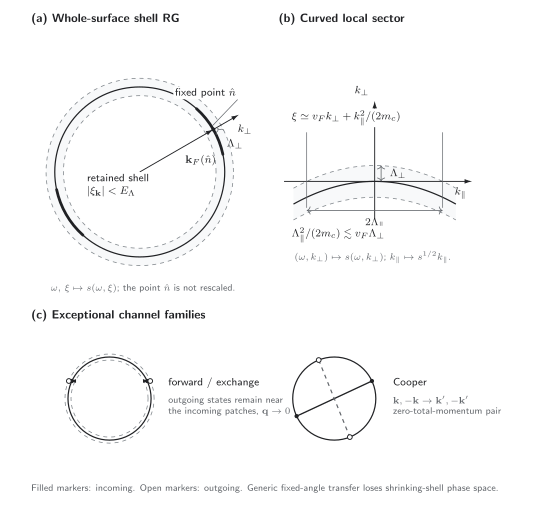
Two distinct low-energy organizations of a smooth, strictly convex two-dimensional Fermi surface and the exceptional four-fermion kinematics they expose. Whole-surface shell RG scales frequency and normal energy while retaining the surface label. A curvature-resolved sector also scales $k_\parallel$, with $\Lambda_\parallel^2/(2m_c)\lesssim v_F\Lambda_\perp$. Forward and exchange configurations keep outgoing states near the incoming patches; the Cooper family maps one antipodal pair into another. The figure is schematic and assumes inversion symmetry, a sharp normal-state pole, nonsingular short-range interactions, nonzero curvature, and no nesting.

Filled markers denote incoming momenta and open markers outgoing momenta. The downloadable SVG and machine-readable semantic record preserve the scaling rules, cutoff relations, encodings, and exclusions.

A patch partition must cover the retained shell exactly once. With equal two-dimensional sectors of full tangential width $2\Lambda_\parallel$ and Fermi-curve length $L_F$,

$$N_{\mathrm{patch}}\simeq \frac{L_F}{2\Lambda_\parallel}.$$

A partition of unity may overlap geometrically, but its weights must sum to one. For a circular surface and sectors near the curvature bound, $N_{\mathrm{patch}}\sim\sqrt{k_F/\Lambda_\perp}$. A distinct whole-surface cell decomposition may choose much narrower cells, for example $\Lambda_\parallel\sim\Lambda_\perp$, and then obtain $N_{\mathrm{patch}}\sim k_F/\Lambda_\perp$. That second count is not the curvature-resolved anisotropic fixed-point scaling used to obtain $-7/4$. Patch number is regulator data. Predictions should stabilize under admissible refinement; changing the number without changing widths and weights consistently creates gaps or double counting.

Momentum conservation selects exceptional channels

Write the antisymmetrized four-point interaction schematically as

$$\begin{aligned} S_4 ={}&\frac14\int\prod_{i=1}^4 \left[\frac{\mathrm d\omega_i\,\mathrm d^d k_i}{(2\pi)^{d+1}}\right] (2\pi)^{d+1}\delta^{(d+1)}(k_1+k_2-k_3-k_4)\\ &\times \Gamma_{a_1a_2;a_3a_4}(1,2;3,4) \bar\psi_{a_3}(3)\bar\psi_{a_4}(4) \psi_{a_2}(2)\psi_{a_1}(1). \end{aligned}$$

If all four fields are expressed in one common local frame and the interaction is a smooth contact vertex, the anisotropic measures, homogeneous conservation delta function, and four fields make that single-patch vertex scale as $s^{(d-1)/2}$. It is naively irrelevant for $d>1$. This is not a global proof for four distinct patch normals: their momentum delta function is not homogeneous under one local frame. The global classification must retain and sum the unscaled surface labels. It then finds reduced shrinking-shell phase space for generic configurations and a different count when momentum conservation becomes geometrically degenerate.

For a regular strictly convex Fermi curve, fixing the total momentum $\mathbf P=\mathbf k_1+\mathbf k_2$ usually makes the intersection of the Fermi curve with its translate by $\mathbf P$ a finite set. The shrinking shell then leaves no continuous internal angular phase space. Two limiting families escape that restriction:

• Forward and exchange scattering. As the transfer $\mathbf q\to0$, each outgoing momentum approaches an incoming patch. The surviving angular function is the Landau interaction $F(\hat n,\hat n')$. Exchanging the two outgoing fermions is fixed by antisymmetry; it is not a second independent coupling. In the regular Fermi-liquid limit, the Wilsonian one-loop beta function of $F$ vanishes, so $F$ labels a fixed-point family. Static and dynamic limits of the associated vertex must still be distinguished.
• Cooper scattering. For an inversion-symmetric surface, $\mathbf P=0$ lets every antipodal pair $(\mathbf k,-\mathbf k)$ scatter into another pair $(\mathbf k',-\mathbf k')$. The resulting kernel $V(\hat n,\hat n')$ must be diagonalized in angular harmonics or lattice point-group form factors.

This geometric classification is derived at tree and one-loop level in Shankar 1994, §§ V–VII, pp. 157–177. In three dimensions the generic on-shell solution set is larger, but the forward and Cooper limits remain the singular families behind the standard weak-coupling Fermi-liquid and pairing flows. In one dimension there is no tangential continuum and generic four-fermion interactions are marginal, so the argument above must be replaced by the right- and left-mover theory.

Let $\nu_{\mathrm{pair}}(0)$ be the density of states for one member of the pair. For a two-spin-degenerate band, the chapter’s total density of states is $N(0)=2\nu_{\mathrm{pair}}(0)$. Normalize the per-species Fermi-surface measure by

$$\mathrm d\mu(\hat n) =\frac{1}{\nu_{\mathrm{pair}}(0)} \frac{\mathrm dS_{\mathbf k}}{(2\pi)^d v_F(\mathbf k)}, \qquad \oint_{\mathrm{FS}}\mathrm d\mu(\hat n)=1,$$

and define the dimensionful Cooper eigenvalue $V_a$ through

$$\oint_{\mathrm{FS}}\mathrm d\mu(\hat n') V(\hat n,\hat n')\phi_a(\hat n') =V_a\phi_a(\hat n).$$

This convention matters on an anisotropic or lattice Fermi surface: using the unnormalized surface measure would make the corresponding eigenvalue already dimensionless. With the normalized measure above, define

$$\lambda_a=\nu_{\mathrm{pair}}(0)V_a, \qquad t=\log\frac{E_0}{E}.$$

With attraction represented by $\lambda_a<0$, the leading logarithmic flow is

$$\frac{\mathrm d\lambda_a}{\mathrm dt}=-\lambda_a^2, \qquad \lambda_a(t)=\frac{\lambda_a(0)}{1+\lambda_a(0)t}.$$

Repulsion approaches zero, while attraction reaches strong coupling at $t_*=1/\lvert\lambda_a(0)\rvert$. The divergence is a stopping signal for the normal-state expansion, not a calculation of the ordered gap, stiffness, or transition. Generic microscopic scattering has not vanished: it matches onto the initial forward and Cooper kernels and onto irrelevant corrections suppressed by powers of $E/E_F$.

For orientation, the chapter’s validity and failure map places these channels beside the tests that can stop the argument, while the claim table records the response and instability assumptions.

A bounded two-dimensional Hubbard application

The square-lattice Hubbard model makes the local-sector bookkeeping concrete. To match the cited theorem exactly, use lattice units and its nearest-neighbor hopping normalization,

$$e_B(\mathbf k)=2-\cos k_x-\cos k_y-\mu_B, \qquad 0<\mu_B<\frac{2-\sqrt2}{2},$$

with on-site interaction $U_B\sum_{\mathbf x}n_{\mathbf x\uparrow}n_{\mathbf x\downarrow}$. Here $U_B$ and the dimensionless temperature $T_B$ are measured in the same hopping unit. In the conventional dispersion $-2t_h(\cos k_x+\cos k_y)-\mu$, the displayed theorem window corresponds to $-4t_h<\mu<-(2+\sqrt2)t_h$. It is deliberately narrower than the full set of smooth convex Fermi curves: the proof also excludes the low-order umklapp configurations it does not control.

Choose a fixed scale ratio $\gamma>1$. On scale $h\leq0$, retain modes with

$$\lvert-ik_0+e_B(\mathbf k)\rvert\asymp\gamma^h$$

and subdivide the annulus into angular sectors of tangential width of order $\gamma^{h/2}$. Curvature then restricts the sector labels that can meet at a vertex. Grassmann determinant bounds control the sum over contractions, while localization separates the renormalizations of the two-point kernel and the marginal part of the four-point kernel.

At temperature $T_B$, fermionic Matsubara frequencies satisfy $\lvert k_0\rvert\geq\pi T_B$, so the flow stops at a finite $h_T$ with $\gamma^{h_T}\asymp T_B$. For sufficiently small $U_B$, Benfatto, Giuliani, and Mastropietro prove convergence and Fermi-liquid control in a window of the form

$$\lvert U_B\rvert\,\lvert\log T_B\rvert\leq c,$$

The resummed multiscale expansion dynamically dresses the propagator, and the theorem shows that the resulting interacting Fermi surface remains regular and convex in this window Benfatto, Giuliani, and Mastropietro 2006, Theorem 1.1 and § 1.4, pp. 813–822. This is a controlled application of the sector picture, but its temperature bound stops at an exponentially small scale. It neither proves the zero-temperature phase nor continues through a Cooper divergence. The rigorous multiscale treatment develops the determinant and sector estimates.

Where the regular-patch argument stops

Situation	Failed step	Required change in conclusion or method
Nested segments	Translated Fermi-surface pieces overlap over a continuum	Finite-wavevector particle–hole channels can become marginal or logarithmic; keep them explicitly
Van Hove point	$v_F=0$ and the normal coordinate is singular	Recenter the scaling at the saddle and retain the enhanced density of states
Inflection or nearly flat region	The quadratic curvature estimate is not uniform	Use the first nonzero tangential derivative and test sector exponents locally
Unscreened long-range force or gapless boson	The four-fermion kernel is not smooth at small transfer	Scale the boson and fermion together; Landau damping and non-Fermi-liquid self-energies may change power counting
Broad or absent fermion pole	$i\omega-\xi$ no longer controls the quadratic fixed point	Determine the interacting propagator and its dynamical exponent before assigning patch dimensions
Inconsistent patch cover	Sector weights do not form a partition of unity	Repair gaps or overlaps before interpreting patch sums; refine the regulator and check stability
Strong-coupling stopping scale	Perturbative vertices become order one	Report a tendency and stop; use a broken-symmetry or nonperturbative continuation for the phase

The next functional-RG page keeps several of these channels coupled and makes regulator, frequency, self-energy, and patch-resolution dependence part of the answer. Pomeranchuk and density-wave instabilities then distinguish uniform shape deformations from finite-wavevector order.

Common pitfalls

Scaling the same tangential variable both ways. A fixed surface label in whole-surface RG and a shrinking coordinate inside one local sector are different variables. Choose the scheme before quoting a field dimension.

Treating the curvature width as an equality. Curvature sets a maximal natural width. Narrower sectors are legitimate, and the patch count changes with that choice.

Calling every microscopic interaction irrelevant. Generic low-energy phase space is suppressed, but its matching contribution survives in the marginal forward and Cooper kernels and in controlled irrelevant corrections.

Reading a divergent Cooper coupling as an ordered phase. The divergence locates the failure of the symmetric weak-coupling flow. It does not determine the ordered-state continuation or prove a material realization.

Exercises

Derive both field dimensions. Reproduce the momentum–frequency scaling of $\psi$ in the whole-surface scheme and in a curvature-resolved sector in $d$ dimensions.

Solution

In the whole-surface scheme, $\mathrm d\omega\,\mathrm d\xi$ scales as $s^2$, the inverse propagator as $s$, and the surface measure does not scale. If $\psi\mapsto s^\alpha\psi$, invariance gives $2+1+2\alpha=0$, hence $\alpha=-3/2$.

In the local scheme, $\mathrm d\omega\,\mathrm dk_\perp\,\mathrm d^{d-1}k_\parallel$ scales as $s^{1+1+(d-1)/2}=s^{(d+3)/2}$. Thus $(d+3)/2+1+2\alpha=0$, giving $\alpha=-(d+5)/4$. For $d=2$, $\alpha=-7/4$.

Estimate a patch count. For a circular quadratic Fermi surface, let $\Lambda_\perp/k_F=10^{-4}$ and choose sectors at the curvature bound. Estimate $\Lambda_\parallel/k_F$ and the number of equal sectors of full width $2\Lambda_\parallel$.

Solution

Since $m_cv_F=k_F$,

$$\frac{\Lambda_\parallel}{k_F} =\sqrt{2\frac{\Lambda_\perp}{k_F}} =\sqrt{2\times10^{-4}} \simeq1.41\times10^{-2}.$$

Using $L_F=2\pi k_F$ gives

$$N_{\mathrm{patch}} \simeq\frac{2\pi k_F}{2\Lambda_\parallel} \simeq2.22\times10^2.$$

The integer used in a calculation would be adjusted so the final weighted sectors cover the curve exactly; the estimate is not universal.

Locate the Cooper degeneracy. For an inversion-symmetric Fermi curve, explain why fixed total momentum $\mathbf P=0$ leaves a continuous family of pairs but a generic nonzero $\mathbf P$ does not.

Solution

At $\mathbf P=0$, choosing any $\mathbf k$ on the Fermi curve automatically places $-\mathbf k$ on it, so the incoming pair is labeled continuously by the position of $\mathbf k$. For generic nonzero $\mathbf P$, both $\mathbf k$ and $\mathbf P-\mathbf k$ must lie on the curve. Geometrically this is the intersection of the curve with its translate by $\mathbf P$, which is a finite set for a regular strictly convex curve. The continuous angular phase space is lost unless the translated curves become degenerate, as in nesting.

Integrate one Cooper eigenchannel. Let $\lambda(0)=-0.20$. Find the leading-logarithmic stopping scale and state the conclusion ceiling.

Solution

The solution is $\lambda(t)=\lambda(0)/[1+\lambda(0)t]$. Its denominator vanishes at $t_*=5$, so $E_*=E_0e^{-5}\simeq6.74\times10^{-3}E_0$. This establishes the scale at which the normal-state weak-coupling expansion fails in that eigenchannel. It does not determine a transition-temperature prefactor, gap magnitude, stiffness, or realized phase.

Find the thermal stop. Why is there no fermionic RG slice with characteristic scale much smaller than $T$ in the finite-temperature Hubbard application?

Solution

Fermionic Matsubara frequencies are $k_0=(2n+1)\pi T_B$, so $\lvert k_0\rvert\geq\pi T_B$. Even on the Fermi surface, $\lvert-ik_0+e_B(\mathbf k)\rvert$ cannot be parametrically below $T_B$. Therefore a slice supported at $\gamma^h\ll T_B$ is empty, and the last nonempty scale satisfies $\gamma^{h_T}\asymp T_B$.

References

• Giuseppe Benfatto, Alessandro Giuliani, and Vieri Mastropietro, “Fermi Liquid Behavior in the 2D Hubbard Model at Low Temperatures,” Annales Henri Poincaré 7 (2006) 809–898, doi:10.1007/s00023-006-0270-z, Open PDF.
• Joseph Polchinski, “Effective Field Theory and the Fermi Surface,” in Recent Directions in Particle Theory, World Scientific (1993) 235–276, doi:10.1142/9789814503577_0001, Open PDF.
• Ramamurti Shankar, “Renormalization-Group Approach to Interacting Fermions,” Reviews of Modern Physics 66 (1994) 129–192, doi:10.1103/RevModPhys.66.129.