

From the Anderson Model to Kondo Exchange
In the local-moment regime, empty and doubly occupied Anderson states are energetically costly but still appear virtually. A Schrieffer–Wolff transformation block-diagonalizes the Hamiltonian so that these charge excursions are represented by operators acting entirely within the singly occupied sector. To second order in hybridization, the result is antiferromagnetic spin exchange plus spin-independent potential scattering.
The transformation is a matching calculation, not an RG flow. It determines a low-energy Hamiltonian, its cutoff, and the corresponding low-energy operators. The exchange runs only after this step, and the construction fails when either charge state is active rather than virtual.
Required background. The Anderson impurity model supplies the atomic sectors, charge gaps, and hybridization convention.
Helpful background. Integrating out heavy fields supplies the distinction between exact elimination and a low-energy expansion.
Separating the charge and spin subspaces
Section titled “Separating the charge and spin subspaces”Write the Anderson Hamiltonian as
with
Let project onto the impurity states and let project onto the empty and doubly occupied sectors. Hybridization is off diagonal between these subspaces:
Choose an anti-Hermitian generator satisfying
Use this generator perturbatively with a finite regulator and a nonresonant retained bath-energy window, for example , where and are the positive removal and addition energies. Higher bath energies are accounted for when matching the parameters of this window. The charge-only projector does not itself separate the spectra of the full metallic Fock-space blocks: at or , hybridization can connect degenerate charge sectors. In an eigenbasis, cannot cancel a nonzero between such states. The following expressions are therefore regulated low-energy matching kernels, not a uniformly bounded unitary block diagonalization across the whole metallic band. The original derivation explicitly discusses the resonant singularity in Schrieffer and Wolff 1966, p. 491, footnote 4.
For the one-orbital model, one explicit choice is
The occupation projectors select the intermediate charge. If the opposite spin is absent, empties the orbital and its low-energy denominator approaches . If the opposite spin is present, the Hermitian-conjugate process creates double occupancy and its cost is .
Expanding the unitary transformation gives
where denotes the charge scale. Projecting the second-order term is equivalent, for a degenerate low-energy sector of energy , to
This form makes the physics transparent: the state leaves , pays a positive excitation energy in , and returns to . The full canonical transformation is systematic; the displayed approximation retains the leading low-energy block. Bravyi, DiVincenzo, and Loss 2011, §2, pp. 2795–2802 gives a modern general formulation of this block diagonalization.
Exchange and scalar scattering
Section titled “Exchange and scalar scattering”Inside the singly occupied subspace, and the impurity bilinear decomposes as
where
Using this identity in separates a spin vector from a scalar. Up to a constant energy shift and a convention-dependent normal-ordering term,
with
Before the low-energy approximation, the exchange amplitude is
and the combined scalar amplitude is
For a local orbital coupled uniformly to bath modes, choose the normalization
The corresponding density of states is normalized per spin and per site,
so and are dimensionless. Stating this normalization is essential when comparing exchange constants across continuum, lattice, and numerical conventions.
For external bath energies small compared with both charge gaps, and , where
Equivalently,
These prefactors use the spin density with . A source that omits the factor from the spin-density definition prints an exchange coefficient smaller by two.
Schrieffer and Wolff 1966, Eqs. (4)–(13), pp. 491–492 performs this transformation in the original Anderson-model convention. The signs above have been translated to the common convention in which in is antiferromagnetic.
Hewson 1993, ch. 1 gives a pedagogical Anderson-to-Kondo derivation and a useful translation among common Hamiltonian conventions.
Why the two virtual paths add in J
Section titled “Why the two virtual paths add in J”The dedicated diagram can now be read as a derivation aid. Start with a singly occupied impurity and an incoming conduction electron of opposite spin. There are two time orderings:
- the impurity electron hops out first, leaving at cost , and the bath electron hops in;
- the bath electron hops in first, creating at cost , and one electron hops out.
Both return to charge one with the two spins exchanged. Fermionic signs and the spin decomposition make their exchange pieces add, whereas their scalar particle and hole pieces have opposite signs.
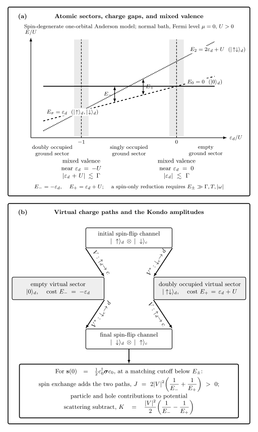
On a narrow screen, swipe the diagram or focus it and use the left/right arrow keys; Home and End move to its edges. Open the full-size diagram.
The two second-order paths through the empty and doubly occupied charge sectors. Their exchange amplitudes add as , while the scalar amplitudes subtract as . For a particle–hole-symmetric bath at , the two costs are equal, so potential scattering vanishes but antiferromagnetic exchange remains. Original schematic for a spin-degenerate orbital and a normal bath; not to scale.
The same information has the following nonvisual form.
| Virtual sector | Energy cost | Contribution to | Contribution to |
|---|---|---|---|
| Empty impurity | |||
| Double impurity |
For , the two-spin energies follow from
The singlet has eigenvalue and the triplet has , so the singlet is lower by . This is the operational meaning of an antiferromagnetic exchange sign.
For a particle–hole-symmetric bath at the symmetric impurity point,
and therefore
The cancellation of is an independent symmetry check. It is not a cancellation of charge fluctuations: both charge sectors still contribute equally to .
Matching scale, errors, and transformed observables
Section titled “Matching scale, errors, and transformed observables”The constant-coupling Kondo model is valid for external energies below both charge gaps. Its natural starting cutoff is of order
with order-one scheme dependence absorbed into how , , and the eventual Kondo scale are defined. Starting a constant- RG flow at a much larger band cutoff double-counts energy ranges in which the Anderson charge states were still dynamical. The next page fixes a density-of-states convention and runs below this matching scale.
The leading control conditions are
If either ratio is order one, the projector has discarded an active state. A small numerical value of a formula for does not rescue the mapping in mixed valence.
Block diagonalization also acts on observables. Every operator must be matched as
For example, the impurity charge is fixed to one at zeroth order inside , but its transformed operator contains virtual bath–impurity pieces whose expectation value records charge fluctuations. A tunnelling operator begins with an composite operator in the Kondo theory. Matching only the Hamiltonian and then using the bare Anderson operator gives incorrect spectroscopy even if the energy spectrum is reproduced.
Nearby orbital multiplets, Hund coupling, spin–orbit coupling, or several conserved bath channels require a larger space. The result may be anisotropic Kondo exchange, Coqblin–Schrieffer exchange, orbital Kondo physics, or additional scalar and tensor operators. A superconducting or pseudogap bath changes the subsequent infrared flow, but it does not remove the requirement that charge elimination be controlled.
The chapter-wide map locates this derivation between Anderson charge dynamics and RG. The displayed one-orbital matching route has one active hybridization eigenchannel and therefore supplies . Genuine screening instead enters through the separate microscopic lane with equivalent conserved baths and channel-resolved exchanges .
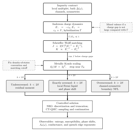
Matching and RG are distinct operations. For the one-orbital route, Schrieffer–Wolff eliminates separated charge sectors and supplies the theory’s , , transformed observables, and starting cutoff. A genuine multichannel route must instead supply and test the channel-resolved and any impurity-spin-assisted off-diagonal exchange. RG then evolves the applicable spin theory; its weak-coupling divergence is a handoff to a nonperturbative fixed-point solution. Original schematic, not to scale.
The impurity claim test matrix records mixed valence and an omitted nearby multiplet as decisive failures of this projection.
Common pitfalls
Section titled “Common pitfalls”Using the right formula in the wrong regime. The denominators can be inserted algebraically even when or is comparable with . In that case the spin-only Hilbert space is not separated and the result is not controlled matching.
Hiding the spin-density convention. Whether is included in changes the printed coefficient called . State the Hamiltonian and compare the dimensionless product only after translating conventions.
Treating matching as the Kondo solution. Positive identifies an antiferromagnetic low-energy interaction. It does not compute the universal strong-coupling phase shift, screening cloud, or Kondo-temperature prefactor.
Forgetting operator matching. A unitary transformation preserves matrix elements only when states and operators are transformed together. Bare impurity charge or tunnelling operators do not act purely inside the Kondo spin space.
Exercises
Section titled “Exercises”1. Detune from particle–hole symmetry. Assume a particle–hole-symmetric bath and energy-independent local hybridization, then put with . Express and in terms of and , and determine their parity under .
Solution
The charge gaps are and . Hence
is even and is odd in the detuning, exactly as particle–hole conjugation requires. Both expressions become unreliable as because one charge gap closes.
2. Recover the antiferromagnetic level ordering. Diagonalize for two spin- degrees of freedom and show which state is lowered for .
Solution
Using ,
For the singlet, and the exchange energy is . For the triplet, and it is . The singlet lies lower by , so is antiferromagnetic in the stated convention.
3. Test a proposed matching. Let , , , and a flat-band cutoff . Find , , and the two charge-control ratios. Would the same mapping be controlled if ?
Solution
For the first point,
so a constant-coupling Kondo description should start no higher than an order-one multiple of , not at the full band cutoff. The ratios are and , giving a reasonably separated moment regime.
At , and . Empty-state fluctuations are active, so the spin-only matching is uncontrolled even though remains much larger than .
References
Section titled “References”- Bravyi, S., DiVincenzo, D. P., and Loss, D. (2011). “Schrieffer–Wolff transformation for quantum many-body systems.” Annals of Physics 326, 2793–2826. doi:10.1016/j.aop.2011.06.004. Open PDF.
- Hewson, A. C. (1993). The Kondo Problem to Heavy Fermions. Cambridge University Press, ch. 1. doi:10.1017/CBO9780511470752.
- Schrieffer, J. R., and Wolff, P. A. (1966). “Relation between the Anderson and Kondo Hamiltonians.” Physical Review 149, 491–492. doi:10.1103/PhysRev.149.491.
Original QFT.org content:CC BY 4.0, unless an item supplies different terms. Third-party material retains its own terms.