Nambu–Gor'kov Green Functions and Anomalous Propagators

Nambu–Gor’kov notation turns the coupled propagation of a fermion and its paired hole into one matrix Dyson problem. For a uniform paired state, that matrix exposes the quasiparticle poles, coherence-factor residues, anomalous propagator, and gap equation in a single calculation. The economy comes with two obligations: every off-diagonal sign belongs to a declared basis and gauge convention, and the particle–hole enlargement must be removed exactly once when states or thermodynamic contributions are counted. This page constructs the method for a balanced, even-parity spin-singlet state and separates its gauge-covariant intermediate quantities from observable spectra and conserving response.

Required background. BCS mean-field theory fixes the uniform saddle and sign of the pairing field. Dyson equations define the self-energy, and Ward-consistent vertices supply the response constraint.

What the four matrix entries mean

Let $\beta=1/T$, let $\omega_n=(2n+1)\pi T$ denote a fermionic Matsubara frequency, and define $\xi_{\mathbf k\sigma}=\varepsilon_{\mathbf k\sigma}-\mu$. Assume equilibrium and translation invariance, with

$$\xi_{\mathbf k\uparrow}=\xi_{-\mathbf k\downarrow} \equiv\xi_{\mathbf k}.$$

The $2\times2$ block below is sufficient for a balanced singlet without spin–orbit mixing. Imbalance, triplet or multiorbital pairing, and broken translation symmetry require a larger kernel or different blocks. The matrices $\tau_{1,2,3}$ below act in the ordered particle–hole space, and $\tau_0$ is its identity. For the spinor

$$\Psi_{\mathbf k} =\begin{pmatrix} c_{\mathbf k\uparrow}\\ c^\dagger_{-\mathbf k\downarrow} \end{pmatrix},$$

define the imaginary-time Green function by

$$\mathcal G(\mathbf k,\tau) =-\langle T_\tau\Psi_{\mathbf k}(\tau) \Psi_{\mathbf k}^\dagger(0)\rangle.$$

We use the fermionic Fourier pair

$$\mathcal G(\mathbf k,\tau) =T\sum_n e^{-i\omega_n\tau}\mathcal G(\mathbf k,i\omega_n), \qquad \mathcal G(\mathbf k,i\omega_n) =\int_0^\beta\!\mathrm d\tau\, e^{i\omega_n\tau}\mathcal G(\mathbf k,\tau),$$

with antiperiodic continuation outside $0\leq\tau<\beta$. Stating this pair is essential: the equal-time regulator below and several anomalous signs change form under a different Fourier convention.

Its entries are

$$\begin{aligned} \mathcal G_{11}(\mathbf k,\tau) &=-\langle T_\tau c_{\mathbf k\uparrow}(\tau) c^\dagger_{\mathbf k\uparrow}(0)\rangle \equiv G(\mathbf k,\tau),\\ \mathcal G_{12}(\mathbf k,\tau) &=-\langle T_\tau c_{\mathbf k\uparrow}(\tau) c_{-\mathbf k\downarrow}(0)\rangle \equiv F(\mathbf k,\tau),\\ \mathcal G_{21}(\mathbf k,\tau) &=-\langle T_\tau c^\dagger_{-\mathbf k\downarrow}(\tau) c^\dagger_{\mathbf k\uparrow}(0)\rangle \equiv \bar F(\mathbf k,\tau),\\ \mathcal G_{22}(\mathbf k,\tau) &=-\langle T_\tau c^\dagger_{-\mathbf k\downarrow}(\tau) c_{-\mathbf k\downarrow}(0)\rangle =-G_\downarrow(-\mathbf k,-\tau). \end{aligned}$$

The last equality uses that antiperiodic continuation when $-\tau$ lies outside the fundamental interval. The diagonal entries propagate a particle and a hole. The off-diagonal entries convert between them through the paired state: $F$ annihilates a pair between its endpoints, while $\bar F$ creates one. Writing the lower-left entry as $F^\dagger$ is common shorthand, but it can be misleading. Hermiticity and Pauli antisymmetry relate $\bar F$ to $F$ through conjugated or reversed arguments and exchanged internal indices; the exact formula depends on the Fourier and index convention. Thus $\bar F(\mathbf k,i\omega_n)$ is not automatically the pointwise complex conjugate of $F(\mathbf k,i\omega_n)$.

The original normal and anomalous equations were introduced in Gor’kov 1958, pp. 505–507, Open PDF. Schrieffer 1999, chs. 7–8 gives a detailed translation between anomalous functions and the Bogoliubov transformation.

Invert the uniform paired propagator

Let $z$ be a complex frequency. On the fermionic Matsubara axis, $z=i\omega_n$. The convention inherited from the preceding page is

$$h_{\mathbf k} =\xi_{\mathbf k}\tau_3 +\operatorname{Re}\Delta\,\tau_1 -\operatorname{Im}\Delta\,\tau_2 =\begin{pmatrix} \xi_{\mathbf k}&\Delta\\ \Delta^*&-\xi_{\mathbf k} \end{pmatrix}.$$

Therefore

$$\mathcal G^{-1}(\mathbf k,z) =z\tau_0-h_{\mathbf k} =\begin{pmatrix} z-\xi_{\mathbf k}&-\Delta\\ -\Delta^*&z+\xi_{\mathbf k} \end{pmatrix}.$$

The determinant and inverse are

$$\begin{aligned} \det\mathcal G^{-1} &=z^2-E_{\mathbf k}^2, & E_{\mathbf k} &=\sqrt{\xi_{\mathbf k}^2+\lvert\Delta\rvert^2},\\ \mathcal G(\mathbf k,z) &=\frac{z\tau_0+h_{\mathbf k}} {z^2-E_{\mathbf k}^2} =\frac1{z^2-E_{\mathbf k}^2} \begin{pmatrix} z+\xi_{\mathbf k}&\Delta\\ \Delta^*&z-\xi_{\mathbf k} \end{pmatrix}. \end{aligned}$$

For the electron entry,

$$G(\mathbf k,z) =\frac{u_{\mathbf k}^2}{z-E_{\mathbf k}} +\frac{v_{\mathbf k}^2}{z+E_{\mathbf k}},$$

where

$$u_{\mathbf k}^2 =\frac12\left(1+\frac{\xi_{\mathbf k}}{E_{\mathbf k}}\right), \qquad v_{\mathbf k}^2 =\frac12\left(1-\frac{\xi_{\mathbf k}}{E_{\mathbf k}}\right).$$

The anomalous entry is

$$F(\mathbf k,z) =\frac{\Delta}{z^2-E_{\mathbf k}^2} =\frac{\Delta}{2E_{\mathbf k}} \left( \frac1{z-E_{\mathbf k}}-\frac1{z+E_{\mathbf k}} \right).$$

An independent way to organize the inversion is the spectral-projector identity

$$\mathcal G(\mathbf k,z) =\frac{P_+(\mathbf k)}{z-E_{\mathbf k}} +\frac{P_-(\mathbf k)}{z+E_{\mathbf k}}, \qquad P_\pm =\frac12\left(\tau_0\pm\frac{h_{\mathbf k}}{E_{\mathbf k}}\right).$$

The checks $P_\pm^2=P_\pm$, $P_+P_-=0$, and $P_++P_-=\tau_0$ test the residues as well as the poles. At large $z$,

$$G=\frac1z+\frac{\xi_{\mathbf k}}{z^2}+O(z^{-3}), \qquad F=\frac{\Delta}{z^2}+O(z^{-4}).$$

These asymptotics are necessary checks, not sufficient ones: reversing the printed sign of both $\Delta$ and $F$ still preserves their powers of $z$.

From Matsubara functions to spectral weights

For the static mean-field kernel, the retarded function follows from $z\to\omega+i0^+$. More generally, analytic continuation is performed only after the frequency-dependent self-energy and its branch structure have been specified. In the gauge where $\Delta>0$ is real, define

$$\mathcal A(\mathbf k,\omega) =i\left[\mathcal G^R(\mathbf k,\omega) -\mathcal G^A(\mathbf k,\omega)\right].$$

The matrix spectral function is

$$\mathcal A(\mathbf k,\omega) =2\pi\left[ P_+\delta(\omega-E_{\mathbf k}) +P_-\delta(\omega+E_{\mathbf k}) \right],$$

so its zeroth moment is the canonical identity,

$$\int_{-\infty}^{\infty} \frac{\mathrm d\omega}{2\pi}\, \mathcal A(\mathbf k,\omega)=\tau_0.$$

The electron spectral function is positive,

$$A_{11}(\mathbf k,\omega) =-2\operatorname{Im}G^R =2\pi\left[ u_{\mathbf k}^2\delta(\omega-E_{\mathbf k}) +v_{\mathbf k}^2\delta(\omega+E_{\mathbf k}) \right],$$

and obeys $\int\mathrm d\omega\,A_{11}/(2\pi)=1$. The real-gauge anomalous component instead has signed weight,

$$\mathcal A_{12}(\mathbf k,\omega) =-2\operatorname{Im}F^R =2\pi\frac{\Delta}{2E_{\mathbf k}} \left[ \delta(\omega-E_{\mathbf k}) -\delta(\omega+E_{\mathbf k}) \right].$$

Consequently,

$$\int\frac{\mathrm d\omega}{2\pi}\mathcal A_{12}=0, \qquad \int\frac{\mathrm d\omega}{2\pi}\,\omega\mathcal A_{12}=\Delta.$$

The first relation is the spectral form of $F(z)\sim z^{-2}$. It also shows why anomalous spectral weight is not a positive probability distribution. The Lehmann and spectral-function page develops the general analytic and positivity framework.

The equal-time limit closes the sign chain back to the gap equation:

$$\begin{aligned} F(\mathbf k,0^-) &=T\sum_n e^{i\omega_n0^+} F(\mathbf k,i\omega_n)\\ &=\langle c_{-\mathbf k\downarrow}c_{\mathbf k\uparrow}\rangle =-\frac{\Delta}{2E_{\mathbf k}} \tanh\frac{E_{\mathbf k}}{2T}. \end{aligned}$$

With the same ultraviolet regulator and matching prescription as on the BCS page,

$$\Delta=-g(\Lambda)\int_{\mathbf k}^{\Lambda}F(\mathbf k,0^-), \qquad g(\Lambda)>0,$$

which reproduces the BCS gap equation. Here the superscript $\Lambda$ means the regulated domain: a reduced-shell model keeps $\lvert\xi_{\mathbf k}\rvert<\omega_c$, whereas a three-dimensional zero-range model must eliminate $g(\Lambda)$ using the scattering-length subtraction. A sign chosen for $\Delta$, the off-diagonal Hamiltonian, or $F$ cannot be changed in isolation.

Gauge covariance and what the anomalous function means

For a neutral system, a constant $\alpha$ labels the global $U(1)$ transformation. For charged matter, use a dimensionless background connection $a_\mu$ and the local convention

$$c(x)\mapsto e^{i\alpha(x)}c(x), \qquad a_\mu(x)\mapsto a_\mu(x)+\partial_\mu\alpha(x).$$

Then

$$\Psi(x)\mapsto e^{i\alpha(x)\tau_3}\Psi(x),$$

and the bilocal matrix transforms covariantly:

$$\mathcal G(x,y)\mapsto e^{i\alpha(x)\tau_3}\mathcal G(x,y) e^{-i\alpha(y)\tau_3}.$$

In particular,

$$F(x,y)\mapsto e^{i[\alpha(x)+\alpha(y)]}F(x,y).$$

For a local pair field $\Delta=\lvert\Delta\rvert e^{i\theta}$,

$$\Delta\mapsto e^{2i\alpha}\Delta, \qquad \theta\mapsto\theta+2\alpha,$$

so $\partial_\mu\theta-2a_\mu$ is invariant. A bilocal charged correlator becomes gauge invariant only after the appropriate Wilson-line or source completion is supplied; a momentum-space $F(\mathbf k,z)$ by itself presupposes the uniform background and gauge convention.

An exact finite system in a fixed-number state has $\langle cc\rangle=0$. The broken-symmetry anomalous function is obtained by taking the thermodynamic limit before sending an auxiliary pair source to zero—the quasiaverage prescription. For a neutral thermodynamic phase in a regime that supports true pair long-range order, the symmetry-preserving statement is off-diagonal long-range order: the two-body density matrix has an eigenvalue proportional to the particle number, equivalently an appropriately projected pair correlation approaches a nonzero long-distance limit. In low-dimensional regimes with only quasi-long-range order, pair correlations instead decay algebraically; stiffness and topological response, not an extensive long-range-order eigenvalue, supply the appropriate criterion. These distinctions and their relation to phase rigidity are developed on the superfluid order and stiffness page. Charged matter additionally requires gauge dressing or a source-complete response. Relative phases between coupled systems can then carry physical content, as can gauge-complete spectra and response functions. The neutral-system distinction is developed by Yang 1962, pp. 694–704; the prohibition on treating a local gauge redundancy as a physical broken symmetry is formalized by Elitzur 1975, pp. 3978–3982.

Change conventions without changing physics

The gauge transformation above is active: it acts on the physical fields and, locally, on the background connection. By contrast, the following operation is a passive coordinate change in Nambu space at fixed physical background. Rephase only the hole component:

$$\widetilde\Psi=U\Psi, \qquad U=\tau_3.$$

Every matrix object must transform, not just one printed symbol:

$$\widetilde{\mathcal G}=U\mathcal G U^\dagger, \qquad \widetilde{\mathcal G}^{-1} =U\mathcal G^{-1}U^\dagger, \qquad \widetilde h=UhU^\dagger.$$

Because $U\tau_{1,2}U^\dagger=-\tau_{1,2}$,

$$\widetilde\Delta=-\Delta, \qquad \widetilde F=-F, \qquad \widetilde{\bar F}=-\bar F,$$

when $\widetilde h$ is written in the same $+\operatorname{Re}\widetilde\Delta\,\tau_1-\operatorname{Im}\widetilde\Delta\,\tau_2$ form. The diagonal entries, determinant, poles, and electron spectral function are unchanged. A disagreement between two printed anomalous signs is therefore not physical until their basis order, hole-component phase, gap definition, and Fourier convention have all been translated.

The convention map makes this covariance visible: follow the two off-diagonal cells through either a constant gauge rotation or the $U=\tau_3$ basis rephasing, then compare the invariant column.

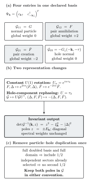
In the declared spin-singlet Nambu basis, diagonal entries propagate a particle or hole and off-diagonal entries annihilate or create a pair. A constant $U(1)$ rotation changes the anomalous phases, while the basis rephasing $U=\tau_3$ reverses their printed signs together with $\Delta$. The determinant and $\pm E_{\mathbf k}$ poles are invariant; particle–hole duplication is removed once according to the declared summation domain. Exact algebraic convention map for a uniform block, not a spacetime diagram.

Download the convention map as SVG or read its semantic record.

A worked residue and convention check

Take a real $\Delta>0$ and one momentum with $\xi_{\mathbf k}=\Delta$. Then

$$(\xi_{\mathbf k}-E_{\mathbf k})u_{\mathbf k} +\Delta v_{\mathbf k}=0, \qquad \frac{v_{\mathbf k}}{u_{\mathbf k}} =\frac{E_{\mathbf k}-\xi_{\mathbf k}}{\Delta}.$$

Together with $u_{\mathbf k}^2+v_{\mathbf k}^2=1$, this direct eigenvector calculation gives

$$E_{\mathbf k}=\sqrt2\,\Delta, \qquad u_{\mathbf k}^2=\frac{2+\sqrt2}{4}, \qquad v_{\mathbf k}^2=\frac{2-\sqrt2}{4}.$$

The two partial-fraction residues are

Pole	$\operatorname{Res}G$	$\operatorname{Res}F$
$+\sqrt2\,\Delta$	$(2+\sqrt2)/4\simeq0.8536$	$+1/(2\sqrt2)\simeq+0.3536$
$-\sqrt2\,\Delta$	$(2-\sqrt2)/4\simeq0.1464$	$-1/(2\sqrt2)\simeq-0.3536$

The normal residues are positive and sum to one; the anomalous residues cancel. The eigenvector calculation therefore gives the same $E$, $u^2$, and $v^2$ as the matrix inverse. After $U=\tau_3$, both anomalous residues reverse sign while the normal residues and poles remain fixed. This is the complete translation test: transform the basis, gap, and Green function together, then compare invariant outputs.

Count particle–hole states once

The poles at $+E$ and $-E$ both belong in the Green function. In the present even-parity singlet block, the basis-specific antiunitary particle–hole operation is

$$\mathcal C=\tau_2\mathsf{K}, \qquad \mathcal C h_{\mathbf k}\mathcal C^{-1}=-h_{-\mathbf k}, \qquad \mathcal C^2=-1,$$

where $\mathsf{K}$ complex conjugates coefficients. The relation follows immediately from $\tau_2\tau_i^*\tau_2=-\tau_i$ for $i=1,2,3$ and the declared evenness under $\mathbf k\mapsto-\mathbf k$. Thus $h_{\mathbf k}\lvert u\rangle=E\lvert u\rangle$ implies $h_{-\mathbf k}\mathcal C\lvert u\rangle=-E\mathcal C\lvert u\rangle$. A larger spin-orbital basis has its own matrix representation of $\mathcal C$; one must not transplant $\tau_2\mathsf{K}$ without transforming the basis. Redundancy is removed when independent states or thermodynamic terms are counted, not by deleting the negative-frequency pole.

Representation	Domain	Counting rule
Reduced block $(c_{\mathbf k\uparrow},c^\dagger_{-\mathbf k\downarrow})^T$	All $\mathbf k$	No extra $1/2$ is inserted; the normal-ordering constant and two positive spin quasiparticles follow the reduced BCS construction.
Fully doubled spin–Nambu basis	Full momentum domain	Write the doubled quadratic form with $1/2$, producing the corresponding $-\tfrac12\operatorname{Tr}\log$ after Gaussian integration, together with the normal-ordering constant.
Any basis restricted to independent particle–hole sectors	Half-domain or one representative per pair	Do not insert a second $1/2$ after the restriction.

Thus “Nambu expressions always carry one half” is false. The correct rule is to declare the basis and summation domain and remove the duplication by exactly one mechanism. Each diagonal spectral function still has its own canonical unit sum rule; $\int\mathrm d\omega\,\operatorname{tr}\mathcal A/(2\pi)=2$ for this $2\times2$ matrix and is not, by itself, evidence of thermodynamic double counting.

At zero energy, $\mathcal C^2=-1$ forces $\lvert u\rangle$ and $\mathcal C\lvert u\rangle$ to be orthogonal partners in this reduced block. A self-conjugate zero mode instead requires a BdG problem whose relevant particle–hole operation squares to $+1$, not merely a change of basis. Class D is one such case when no additional antiunitary or chiral symmetry is present; the full symmetry class also depends on time-reversal and spin-rotation symmetries. The topological boundary-mode page develops when such zero modes occur and how they are counted.

Interacting Dyson equation and conserving response

For $k=(i\omega_n,\mathbf k)$, define two different reversed arguments,

$$\bar k=(-i\omega_n,-\mathbf k), \qquad k^\dagger=(-i\omega_n,\mathbf k).$$

The first reverses frequency and momentum; the second is the equilibrium analytic-reflection argument at fixed momentum. Choose the normal reference propagator and define the Nambu self-energy by

$$\mathcal G^{-1}(k) =\mathcal G_0^{-1}(k)-\Sigma_{\mathrm N}(k) =\begin{pmatrix} i\omega_n-\xi_{\mathbf k}-\Sigma_{11}(k)&-\Phi(k)\\ -\bar\Phi(k)&i\omega_n+\xi_{\mathbf k}-\Sigma_{22}(k) \end{pmatrix}.$$

$\Phi$ and $\bar\Phi$ are anomalous self-energies, but the four displayed entries are not four arbitrary functions. In this balanced even-parity singlet block, Pauli antisymmetry and Nambu redundancy require

$$\begin{aligned} \mathcal G(k)&=-\tau_2\mathcal G^T(\bar k)\tau_2,\\ \Sigma_{\mathrm N}(k)&=-\tau_2\Sigma_{\mathrm N}^T(\bar k)\tau_2, \end{aligned}$$

and therefore

$$\Sigma_{22}(k)=-\Sigma_{11}(\bar k), \qquad \Phi(k)=\Phi(\bar k), \qquad \bar\Phi(k)=\bar\Phi(\bar k).$$

Before the antisymmetric spin-singlet tensor is factored out, the corresponding Pauli relation is $\Phi_{\alpha\beta}(k)=-\Phi_{\beta\alpha}(\bar k)$. Conjugation is a separate condition: equilibrium analytic reflection gives

$$\Sigma_{\mathrm N}(k)^\dagger =\Sigma_{\mathrm N}(k^\dagger), \qquad \bar\Phi(\mathbf k,i\omega_n) =\Phi(\mathbf k,-i\omega_n)^*.$$

For even-frequency pairing, the latter becomes the pointwise relation $\bar\Phi=\Phi^*$; a real-gap gauge further makes the two entries equal. Larger spin-orbital or triplet kernels require their full charge-conjugation matrix and index-exchange rule instead of these scalar formulas.

After analytic continuation, isolated sharp quasiparticle poles solve $\det\mathcal G^{-1}(\mathbf k,z)=0$ on the appropriate continued sheet. The physical spectral gap is instead the onset of support of a measured diagonal spectral function and may end at a continuum threshold rather than an isolated pole. Neither quantity need equal the magnitude of one off-diagonal self-energy entry.

Define a pairing kernel $K_{pp}$ by the closure

$$\Phi(k) =-T\sum_{n'}\int_{\mathbf k'} K_{pp}(k,k')F(k'),$$

with $K_{pp}=g(\Lambda)>0$ on the regulated domain in the instantaneous contact convention used above. Other authors absorb this minus sign into a signed irreducible vertex. A frequency-dependent or momentum-dependent closure must specify its integration measure, internal indices, ultraviolet matching, and approximation. Self-consistency alone does not make that approximation controlled.

Gauge invariance imposes a second constraint. For an external bosonic transfer $q=(i\Omega_m,\mathbf q)$, let $\Gamma^\mu(k+q,k)$ be the full amputated electromagnetic vertex. Let $Q=\tau_3$ be the Nambu charge generator and absorb the probe-charge sign into the vertex definition. The superconducting Ward identity can be written

$$q_\mu\Gamma^\mu(k+q,k) =\mathcal G^{-1}(k+q)Q -Q\mathcal G^{-1}(k).$$

The anomalous self-energy does not commute with $Q$. Consequently, even as $q\to0$, the right-hand side retains the phase-sector contribution that the compatible vertex must reproduce. A dressed Nambu bubble with an unrelated bare vertex is not a gauge-invariant electromagnetic response. Nambu 1960, §§III–IV derives this generalized Ward construction; Baym and Kadanoff 1961, pp. 291–295 gives the general self-energy/vertex consistency principle.

Retarded electron–phonon closure belongs to Eliashberg theory. The phase-sector vertex and its collective poles are developed on the collective-mode page.

Diagnostics and stop conditions

Use several independent checks; no single one detects every convention error.

Check	Required result	Stop condition
Normal limit	$\Delta,\Phi\to0$ recovers the declared normal propagator	A diagonal sign, momentum reversal, or normal-state pole is wrong.
Matrix algebra	Direct inverse, determinant, projectors, and Bogoliubov eigenvectors agree	Poles or residues differ between the two routes.
High-frequency and spectral moments	$G\sim z^{-1}$, $F\sim z^{-2}$, $\int A_{11}/(2\pi)=1$, and $\int \mathcal A_{12}/(2\pi)=0$ in the real gauge	Canonical anticommutation or the anomalous sign structure fails.
Particle–hole map	$\mathcal C h_{\mathbf k}\mathcal C^{-1}=-h_{-\mathbf k}$ in the declared basis, with matched $\pm E$ eigenvectors	A partner is missing, duplicated, or mapped with the wrong momentum.
Convention covariance	A complete basis or gauge transformation changes $\Delta$, $F$, and vertices together but leaves invariant outputs fixed	A claimed pole, density, or response changes under a pure reparametrization.
Counting declaration	Basis, momentum domain, normal-ordering constant, and one de-duplication rule are explicit	An unexplained $1/2$ or missing sector remains.
Retarded causality	No physical retarded pole lies in the upper half-plane; diagonal spectral weight is nonnegative	The continuation or self-energy violates causality.
Conserving response	The self-energy and vertex satisfy the Nambu Ward identity and applicable sum rules	Do not interpret the electromagnetic kernel or a collective pole.

The shared chapter map places this method between the paired saddle and three distinct downstream calculations: spatial BdG spectra, collective fluctuations, and phase response. It does not make any of those later claims automatically.

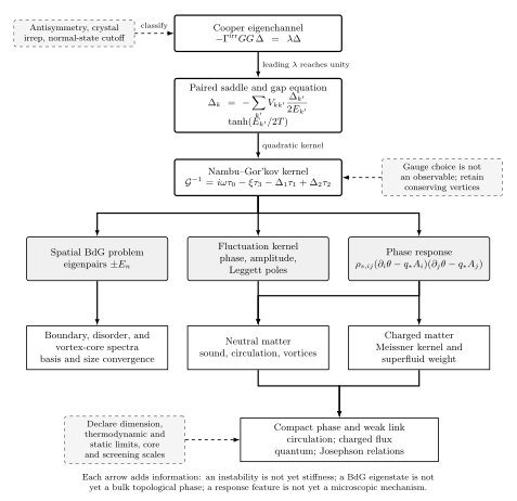
Nambu notation is the matrix dictionary between a paired saddle and later calculations, not an additional physical degree of freedom. The diagram’s arrows show which new inputs are needed before spatial spectra, collective poles, stiffness, or electromagnetic response can be inferred. Original schematic, not to scale.

Read the chapter map’s semantic record. The paired-matter claim test matrix gives the corresponding observable ceilings.

Common pitfalls

Treating $F$ as a measured condensate density. $F$ is a gauge-covariant, convention-dependent amplitude. Observable claims require a gauge-complete source, relative phase, spectrum, or response function.

Comparing anomalous signs before translating conventions. A hole-component rephasing reverses $F$ and $\Delta$ together. Compare determinants, poles, and translated observables only after mapping the full basis and Fourier convention.

Inserting a universal factor of one half. The factor belongs to a particular doubled basis and domain. A reduced block or restricted domain may already have removed the redundancy.

Calling a self-consistent approximation conserving. Iterating Dyson’s equation does not ensure the matching Ward vertex. Test the identity and sum rules explicitly.

Deleting the negative-frequency pole. Both poles are required for the electron spectral function and its unit sum rule. Particle–hole redundancy is a state-counting issue, not permission to alter the analytic propagator.

Exercises

1. Recover the matrix spectral sum rule. For real $\Delta$, verify $P_\pm^2=P_\pm$, $P_+P_-=0$, and $P_++P_-=\tau_0$. Use the projectors to derive $\mathcal A$ and its zeroth moment. Why does $\int\mathrm d\omega\,\operatorname{tr}\mathcal A/(2\pi)=2$ not determine a thermodynamic factor of one half?

Solution

Since $h_{\mathbf k}^2=E_{\mathbf k}^2\tau_0$,

$$P_\pm^2 =\frac14\left(\tau_0\pm\frac{h}{E}\right)^2 =\frac12\left(\tau_0\pm\frac{h}{E}\right) =P_\pm.$$

The same identity gives $P_+P_-=0$ and direct addition gives $P_++P_-=\tau_0$. Continuing $z\to\omega+i0^+$ and using $-2\operatorname{Im}(\omega-E+i0^+)^{-1}=2\pi\delta(\omega-E)$ yields

$$\mathcal A =2\pi\left[P_+\delta(\omega-E)+P_-\delta(\omega+E)\right].$$

Integrating gives $P_++P_-=\tau_0$. The trace is therefore two because the matrix has two canonical diagonal components. It does not decide the thermodynamic factor: that factor follows separately from the declared basis, momentum domain, and de-duplication mechanism.

2. Recover the gap equation from the anomalous propagator. Evaluate the Matsubara sum for $F(\mathbf k,0^-)$ and insert it into $\Delta=-g(\Lambda)\int_{\mathbf k}^{\Lambda}F(\mathbf k,0^-)$. Which quantities change sign if the hole component is rephased by $\tau_3$?

Solution

On the Matsubara axis,

$$F(\mathbf k,i\omega_n) =-\frac{\Delta}{\omega_n^2+E_{\mathbf k}^2}.$$

Using

$$T\sum_n\frac1{\omega_n^2+E^2} =\frac1{2E}\tanh\frac{E}{2T}$$

gives

$$F(\mathbf k,0^-) =-\frac{\Delta}{2E_{\mathbf k}} \tanh\frac{E_{\mathbf k}}{2T}.$$

Therefore a nonzero saddle obeys

$$\frac1{g(\Lambda)} =\int_{\mathbf k}^{\Lambda}\frac1{2E_{\mathbf k}} \tanh\frac{E_{\mathbf k}}{2T}.$$

Under $U=\tau_3$, both the printed $F$ and the gap coordinate change sign. The gap equation is unchanged because its two convention-dependent sides transform together. Removing $\Lambda$ requires the same coupling renormalization as in the main text.

3. Find the missing phase vertex. Insert

$$\mathcal G^{-1}(k) =i\omega_n\tau_0-\xi_{\mathbf k}\tau_3-\Delta\tau_1$$

with real $\Delta$ into the Ward identity at $q=(i\Omega_m,\mathbf0)$. Show why the bare density vertex $Q=\tau_3$ is insufficient.

Solution

The right-hand side is

$$\begin{aligned} \mathcal G^{-1}(k+q)Q-Q\mathcal G^{-1}(k) &=i\Omega_m\tau_3 -\Delta[\tau_1,\tau_3]\\ &=i\Omega_m\tau_3+2i\Delta\tau_2. \end{aligned}$$

A bare density vertex supplies only the first term. The second is a phase-direction rotation of the anomalous self-energy. The full vertex must contain the compatible order-parameter or collective contribution so that its contraction with $q_\mu$ reproduces this term. A bubble with the paired propagator but only the bare vertex therefore fails the superconducting Ward identity.

The reusable workflow is therefore: declare the Nambu basis, Fourier pair, and independent momentum domain; construct and invert the kernel; continue it and test its spectral moments; transform every matrix entry together when changing conventions; remove particle–hole duplication exactly once; and pair a dressed self-energy with its compatible vertex before interpreting response.

Continue

Bogoliubov–de Gennes theory promotes the uniform matrix to a spatial eigenproblem with boundaries and self-consistency. Phase, amplitude, and Leggett modes build the consistent two-particle fluctuation kernel. Eliashberg theory develops frequency-dependent normal and anomalous self-energies.

References

• Baym, G., and Kadanoff, L. P. (1961). “Conservation laws and correlation functions.” Physical Review 124, 287–299. doi:10.1103/PhysRev.124.287.
• Elitzur, S. (1975). “Impossibility of spontaneously breaking local symmetries.” Physical Review D 12, 3978–3982. doi:10.1103/PhysRevD.12.3978.
• Gor’kov, L. P. (1958). “On the energy spectrum of superconductors.” Soviet Physics JETP 7, 505–508. Open PDF.
• Nambu, Y. (1960). “Quasi-particles and gauge invariance in the theory of superconductivity.” Physical Review 117, 648–663. doi:10.1103/PhysRev.117.648.
• Schrieffer, J. R. (1999). Theory of Superconductivity, revised edition. Westview Press. Publisher record.
• Yang, C. N. (1962). “Concept of off-diagonal long-range order and the quantum phases of liquid He and of superconductors.” Reviews of Modern Physics 34, 694–704. doi:10.1103/RevModPhys.34.694.