Functional RG for Competing Fermi-Surface Instabilities

Functional renormalization group (fRG) is useful when the same low-energy fermions can reinforce several candidate orders. It evolves one regulated many-body vertex while retaining the particle–particle and both particle–hole loop geometries, then projects the result onto pairing, magnetic, charge, and Fermi-surface-deformation responses. The reliable output is a tendency whose symmetry and ordering remain stable under declared refinements, together with the scale at which the normal-state approximation loses control. A large vertex entry, by itself, is neither a susceptibility nor proof of an ordered phase.

This page specializes to spin-$1/2$ lattice fermions in a translation-invariant normal state, with the two-dimensional weakly repulsive Hubbard model as the worked case. Frequencies are Euclidean Matsubara frequencies, the interaction is short-ranged, and the flow starts in weak coupling. Nesting and van Hove points are allowed as resolved features of the discretization, but they weaken the regular curved-surface estimates that justify a simple truncation. Strong bare coupling, a destroyed fermion pole, and the ordered state lie outside the controlled scope.

Required background. Fermi-surface patch scaling supplies the surface measure, patch weights, and weak-coupling channel kinematics. The general functional-RG construction supplies the effective average action and exact hierarchy. Helpful background. Functional-method validation organizes regulator, truncation, and benchmark tests.

A fermionic flow with a declared sign convention

Let $k=(i\omega,\mathbf k)$ and add the quadratic regulator

$$\Delta S_\Lambda =\sum_{k,a}\bar\psi_a(k)R_\Lambda(k)\psi_a(k).$$

For the exact functional identity, collect the independent Grassmann fields into the doubled vector $\Psi=(\psi,\bar\psi^{\mathsf T})^{\mathsf T}$. Let $\boldsymbol\Gamma_\Lambda^{(2)}$ be the full left/right Hessian in this doubled space and let $\boldsymbol{\mathcal R}_\Lambda$ be the corresponding antisymmetric regulator matrix. With the regulator term subtracted in the definition of the effective average action,

$$\partial_\Lambda\Gamma_\Lambda[\bar\psi,\psi] =-\frac12\operatorname{Tr}\!\left[ \bigl(\boldsymbol\Gamma_\Lambda^{(2)}+\boldsymbol{\mathcal R}_\Lambda\bigr)^{-1} \partial_\Lambda\boldsymbol{\mathcal R}_\Lambda \right].$$

The minus sign is the fermionic supertrace sign and the factor $1/2$ compensates the doubled field space; field-independent normalization terms have been omitted. At nonzero Grassmann background the $\psi\psi$ and $\bar\psi\bar\psi$ Hessian blocks need not vanish, so replacing the matrix Hessian by only $\delta^2\Gamma_\Lambda/(\delta\psi\,\delta\bar\psi)$ is not the exact functional equation. The normal-state zero-field blocks may be reduced only after the functional derivatives that generate the vertex hierarchy have been taken. Choose $\boldsymbol{\mathcal R}_{\Lambda_0}$ so that fluctuations are frozen at the ultraviolet scale $\Lambda_0$, set $\Gamma_{\Lambda_0}$ by the microscopic action, and lower $\Lambda$ until $\boldsymbol{\mathcal R}_{\Lambda\to0}\to0$. The exact identity and its fermionic conventions are derived in Metzner et al. 2012, § II.B–C, Eqs. (35)–(52), pp. 306–310.

For a normal state, expand the scale-dependent action as

$$\begin{aligned} \Gamma_\Lambda={}& \sum_{1,2}\bar\psi_1 \bigl[G_0^{-1}-\Sigma_\Lambda\bigr]_{12}\psi_2\\ &+\frac14\sum_{1,2,3,4} \Gamma_\Lambda^{(4)}(1,2;3,4) \bar\psi_3\bar\psi_4\psi_2\psi_1 +\Gamma_\Lambda^{(6)}+\cdots . \end{aligned}$$

The labels include momentum, frequency, spin, and band or orbital indices. We take $1,2$ as incoming and $3,4$ as outgoing, so $k_1+k_2=k_3+k_4$. The four-point vertex is antisymmetric under $1\leftrightarrow2$ and separately under $3\leftrightarrow4$. The regulated dressed and single-scale propagators are

$$G_\Lambda =\bigl[G_0^{-1}+R_\Lambda-\Sigma_\Lambda\bigr]^{-1}, \qquad S_\Lambda =-G_\Lambda(\partial_\Lambda R_\Lambda)G_\Lambda,$$

where $S_\Lambda$ differentiates the regulator at fixed self-energy. Consequently,

$$\partial_\Lambda G_\Lambda =S_\Lambda +G_\Lambda(\partial_\Lambda\Sigma_\Lambda)G_\Lambda.$$

With the external-leg convention above, the self-energy contraction is

$$\partial_\Lambda\Sigma_\Lambda(3;1) =\sum_{2,4}S_\Lambda(2,4) \Gamma_\Lambda^{(4)}(1,2;3,4).$$

All sums include the appropriate momentum, Matsubara-frequency, and internal-index measure. Dropping $\Gamma_\Lambda^{(6)}$ closes the usual level-two hierarchy. For a bare two-body interaction it reproduces the four-point beta function through $O(U^2)$; omitted six-point feedback begins at $O(U^3)$ even though the closed equations resum selected terms to all orders. The Katanin substitution replaces $S_\Lambda$ by the total derivative $\partial_\Lambda G_\Lambda$ inside the vertex loops. It therefore requires a computed self-energy flow. It adds a specific self-energy-insertion and higher-loop contribution and improves Ward-identity behavior, but it is not the full six-point vertex or a general proof of conservation Katanin 2004, pp. 3–4.

Three transfers, one reconstructed vertex

Three bosonic transfers organize the one-loop contractions:

$$P=k_1+k_2, \qquad Q=k_3-k_1, \qquad Q'=k_4-k_1.$$

$P$ is the total momentum and frequency of the incoming pair; $Q$ and $Q'$ are the two inequivalent particle–hole transfers. With the external-leg ordering fixed above, the exact four-point hierarchy has the structure

$$\partial_\Lambda\Gamma_\Lambda^{(4)} =\mathcal T_{\mathrm{pp},\Lambda}(P) +\mathcal T_{\mathrm{ph,d},\Lambda}(Q) +\mathcal T_{\mathrm{ph,cr},\Lambda}(Q') +\mathcal R_\Lambda^{(6)}.$$

Here $\mathcal R_\Lambda^{(6)}$ denotes the six-point contribution; the level-two truncation sets it to zero. To make the signs and crossings reproducible, introduce internal labels $a,a',b,b'$ and define

$$\left.\partial_\Lambda\Gamma_\Lambda^{(4)}(1,2;3,4) \right|_{(\Gamma^{(4)})^2} =\sum_{a,a',b,b'}G_\Lambda(a,a')S_\Lambda(b,b') \bigl(\mathcal P-\mathcal D+\mathcal C\bigr),$$

where

$$\begin{aligned} \mathcal P={}& \Gamma_\Lambda^{(4)}(a,b;3,4) \Gamma_\Lambda^{(4)}(1,2;a',b'),\\ \mathcal D={}& \Gamma_\Lambda^{(4)}(1,a;3,b') \Gamma_\Lambda^{(4)}(b,2;a',4) +(a\leftrightarrow b,\ a'\leftrightarrow b'),\\ \mathcal C={}& \Gamma_\Lambda^{(4)}(1,a;4,b') \Gamma_\Lambda^{(4)}(b,2;a',3) +(a\leftrightarrow b,\ a'\leftrightarrow b'). \end{aligned}$$

$\mathcal P$, $\mathcal D$, and $\mathcal C$ are respectively the particle–particle, direct particle–hole, and crossed particle–hole contractions in this leg ordering; their distinguished external transfers are $P$, $Q$, and $Q'$. The six-point remainder is $-\sum_{a,a'}S_\Lambda(a,a')\Gamma_\Lambda^{(6)}(1,2,a;3,4,a')$. These formulas are the index form of Metzner et al. 2012, Eq. (52), pp. 309–310. In a Katanin flow, each $S_\Lambda$ in the quadratic-vertex terms is replaced by $\partial_\Lambda G_\Lambda$; dummy-index symmetries and the explicitly exchanged terms account for the derivative placement on the partner line. Thus an enhancement first visible at an antiferromagnetic transfer is fed back into the Cooper and forward-scattering projections at the next step; the channels are not independent differential equations.

The exact parquet decomposition is

$$\Gamma_\Lambda^{(4)} =\Lambda_{\mathrm{2PI},\Lambda} +\Phi_{\mathrm{pp},\Lambda} +\Phi_{\mathrm{ph},\Lambda} +\Phi_{\overline{\mathrm{ph}},\Lambda},$$

where $\Lambda_{\mathrm{2PI},\Lambda}$ is fully two-particle irreducible and each $\Phi$ carries one reducible channel. Replacing $\Lambda_{\mathrm{2PI},\Lambda}$ by $\Gamma_{\mathrm{bare}}^{(4)}$ defines the first-order parquet approximation; it is not an exact identity for the Hubbard model. The diagrammatic assignment of a reducible diagram to particle–particle, direct particle–hole, or crossed particle–hole class is unique. What remains convention-dependent at finite resolution is the allocation of smooth remainders, the Fierz or bosonization basis, and the projection of unresolved momentum and frequency structure. Assign every differentiated diagram once, preserve antisymmetry and crossing, and reconstruct $\Gamma_\Lambda^{(4)}$ before computing observables. The channel construction and its residual parametrization ambiguity are explicit in Husemann and Salmhofer 2009, §§ 2–4, pp. 3–13.

The figure summarizes this coupled logic. In the upper panel, follow the common full vertex through all three loop transfers and back into its derivative. In the lower panel, follow projected responses through the refinement gates before reading the endpoint.

On a narrow screen, swipe or use the Left and Right arrow keys to pan across the figure. Home and End move to its edges. A full-size link is also available.

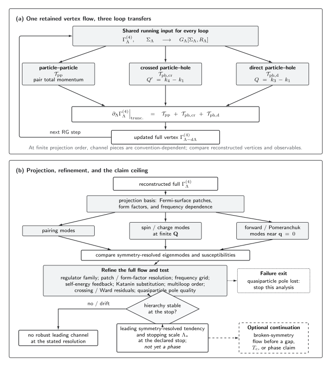
Coupled normal-state fRG workflow and its conclusion ceiling. The upper panel is schematic: particle–particle and the two particle–hole loop classes use the same reconstructed four-point vertex, while $\Sigma_\Lambda$ changes every internal $G_\Lambda$. Reducibility classes are exact diagrammatic categories, but replacing the fully irreducible vertex by the bare interaction and projecting onto finite form-factor, frequency, or patch bases are approximations. The lower panel separates a stable leading response and approximation-dependent stopping scale $\Lambda_*$ from an unresolved hierarchy or a failed fermion-pole assumption. Neither branch proves an ordered phase; a gap, transition, or coexistence claim requires a controlled continuation below the symmetric-flow stop.

The downloadable SVG and machine-readable semantic record preserve the transfer definitions, arrow meanings, validation gates, and inference limits. This compact table supplies the same relations without requiring the image.

Flow object	Resolved transfer or projection	Data that must be retained	Convergence question	Invalid inference
Particle–particle loop	Pair total $P$	Relative momenta, frequencies, spin parity	Does the pairing eigenfunction stabilize?	One attractive entry proves superconductivity
Crossed particle–hole loop	Transfer $Q'$	Spin/charge tensor and finite-$Q'$ structure	Do magnetic or density peaks survive refinement?	A large vertex component is a susceptibility
Direct particle–hole loop	Transfer $Q$	Forward and exchange limits, crossing partners	Are uniform and finite-$Q$ limits separated?	Every forward enhancement is nematic order
Reconstructed $\Gamma_\Lambda^{(4)}$	All three transfers	Smooth remainder and every retained basis coefficient	Are crossing and antisymmetry residuals small?	Channel pieces may be compared without reconstruction
Physical response	Source vertex or Bethe–Salpeter kernel	Bubble weights, operator normalization, and wave vector	Is the response hierarchy stable across admissible schemes?	$\Lambda_*$ is a transition temperature

Patches, form factors, and frequency data

On a regular Fermi surface, with finite nonzero $v_F$ and finite density of states, an $N$-patch calculation replaces the surface by weighted cells. Reuse the per-species normalized measure from the patch-theory page,

$$\mathrm d\mu(\hat n) =\frac{1}{\nu_{\mathrm{pair}}(0)} \frac{\mathrm dS_{\mathbf k}}{(2\pi)^d v_F(\mathbf k)}, \qquad \oint_{\mathrm{FS}}\mathrm d\mu=1,$$

and define

$$w_i=\int_{\mathcal P_i}\mathrm d\mu, \qquad \sum_iw_i=1.$$

Patch values are quadrature data, not equally weighted angular samples. These formulas do not apply at a van Hove saddle, where $v_F=0$ and $\nu_{\mathrm{pair}}(0)$ diverges. There, retain finite-$\Lambda$ or finite-$T$ momentum-and-energy cells and form the channel bubble directly, for example

$$\chi^{0,X}_{mn}(q;\Lambda,T) =\frac{T}{N_s}\sum_{\omega_n,\mathbf k} f_m^*(\mathbf k)\, \mathcal B_X[G_\Lambda](k,q)\, f_n(\mathbf k),$$

with the particle–particle or particle–hole propagator product $\mathcal B_X$ and its channel sign declared. This finite-shell quadrature, not normalization by $\nu_{\mathrm{pair}}(0)$, is the appropriate basis for the van-Hove benchmark.

On a regular surface, a point-group form-factor basis obeys

$$\sum_iw_i f_\alpha^*(i)f_\beta(i)=\delta_{\alpha\beta}.$$

In a channel decomposition one writes, for example,

$$\Phi_{X,\Lambda}(k,k';q) \simeq \sum_{m,n}f_m(k)B^X_{mn,\Lambda}(q)f_n^*(k'),$$

while keeping the bosonic transfer $q$ on a sufficiently fine grid. The fermionic radial and frequency variables must either remain explicit or be removed by a declared projection. “Static vertex on the Fermi surface” is a substantial approximation near a van Hove point or when self-energy structure develops; it is not a harmless change of notation.

For a singlet Cooper diagnostic on that regular surface, a convenient dimensionless weighted kernel is

$$K^{\mathrm{pp}}_{ij} =-\nu_{\mathrm{pair}}(0) \sqrt{w_i}\,V^{\mathrm{pp}}_{ij}\sqrt{w_j}, \qquad \sum_jK^{\mathrm{pp}}_{ij}\varphi_j =\lambda_{\mathrm{pp}}\varphi_i.$$

The minus sign makes an attractive pairing direction positive in this convention. Do not multiply by the density of states twice: it is outside the normalized $w_i$. Particle–hole kernels contain their own bubble and spin or charge factors, so their raw eigenvalues are not numerically comparable to $\lambda_{\mathrm{pp}}$. State each operator normalization and compare physical responses.

From a vertex to competing responses

Let $N_s$ be the number of lattice sites. Normalize the static Fourier operators by $N_s^{-1/2}$ so that their connected susceptibilities are intensive:

$$\begin{aligned} \widehat\Delta_f(\mathbf P) &=\frac1{\sqrt{N_s}}\sum_{\mathbf k}f(\mathbf k) c_{\mathbf k,\uparrow} c_{\mathbf P-\mathbf k,\downarrow},\\ \widehat S_f^a(\mathbf Q) &=\frac1{2\sqrt{N_s}} \sum_{\mathbf k,\alpha,\beta}f(\mathbf k) c^\dagger_{\mathbf k+\mathbf Q,\alpha} \sigma^a_{\alpha\beta}c_{\mathbf k,\beta},\\ \widehat\rho_f(\mathbf Q) &=\frac1{\sqrt{N_s}}\sum_{\mathbf k,\alpha}f(\mathbf k) c^\dagger_{\mathbf k+\mathbf Q,\alpha}c_{\mathbf k,\alpha}. \end{aligned}$$

$\widehat\rho_f(\mathbf0)$ is a general forward or Pomeranchuk probe. It is nematic only when $f$ belongs to a point-group-breaking representation such as $B_{1g}$ or $B_{2g}$; an $A_{1g}$ extended-$s$ form factor preserves the lattice symmetry. $\widehat S_f^a(\pi,\pi)$ probes commensurate antiferromagnetism, and $\widehat\Delta_f(\mathbf0)$ probes zero-momentum pairing. Their connected susceptibility matrix is

$$\chi^X_{mn}(q) =\int_0^\beta\mathrm d\tau\, \left\langle \widehat O^X_m(\mathbf q,\tau) \widehat O^{X\dagger}_n(\mathbf q,0) \right\rangle_c.$$

For internal Matsubara loops, $\sum_k$ below means $(T/N_s)\sum_{\omega_n,\mathbf k}$; this convention must accompany any exported response data. There are two consistent routes. At conventional level two or one loop, one can flow the three-point source vertices $h^X_\Lambda$ and $\chi^X_\Lambda$ together with $\Sigma_\Lambda$ and $\Gamma_\Lambda^{(4)}$. Their structure is

$$\partial_\Lambda h^X_\Lambda =\Gamma^X_\Lambda\circ\dot\Pi^X_\Lambda\circ h^X_\Lambda, \qquad \partial_\Lambda\chi^X_\Lambda =h^{X\dagger}_\Lambda\circ\dot\Pi^X_\Lambda\circ h^X_\Lambda,$$

where $h^X_{\Lambda_0}$ is the chosen form factor, $\chi^X_{\Lambda_0}=0$, and the channel definition absorbs the necessary fermion-loop, spin, and charge signs. Alternatively, one can solve a Bethe–Salpeter equation with $I_X$, the vertex irreducible in channel $X$. In a static Hermitian source basis, absorb the channel sign into $I_X$ and define

$$K_X=\bigl(\chi_X^0\bigr)^{1/2} I_X\bigl(\chi_X^0\bigr)^{1/2}.$$

Then

$$\chi_X =\bigl(\chi_X^0\bigr)^{1/2} (1-K_X)^{-1} \bigl(\chi_X^0\bigr)^{1/2}.$$

An eigenvalue $\lambda_X\to1$ of this $K_X$ signals a response singularity within that convention and approximation. If post-processing instead uses the full channel vertex $F_X$, contract it directly,

$$\chi_X=\chi_X^0+\chi_X^0\circ F_X\circ\chi_X^0,$$

with the same declared signs; inserting $F_X$ into a second ladder equation would double count channel-reducible diagrams. The bubble $\chi_X^0$, source vertices, transfer, temperature, and form-factor normalization are part of the observable. Halboth and Metzner derive explicit source-vertex and susceptibility flows in Halboth and Metzner 2000, § II.C, Eqs. (43)–(46), pp. 6–7. At multiloop convergence, flowing-source and post-processed response routes agree within the chosen parquet approximation only when the corresponding multiloop corrections to the fermion–boson vertex and susceptibility flow are included; inserting a multiloop $\Gamma^{(4)}$ into the displayed one-loop response equations is not sufficient Tagliavini et al. 2019, § 2.2, Eqs. (23)–(26).

A historical weak-coupling Hubbard benchmark

Consider

$$\mathcal K=H-\mu N =\sum_{\mathbf k,a}\xi_{\mathbf k} c_{\mathbf k a}^\dagger c_{\mathbf k a} +U\sum_{\mathbf x}n_{\mathbf x\uparrow}n_{\mathbf x\downarrow}, \qquad U>0,$$

with

$$\xi_{\mathbf k} =-2t(\cos k_x+\cos k_y) -4t'\cos k_x\cos k_y-\mu.$$

The van Hove level is $\mu=4t'$ in this convention. A calculation must state $U/t$, $t'/t$, $\mu/t$ or density, $T/t$, whether density or chemical potential is held fixed, the regulator and $\Lambda_0$, patch weights or form factors, frequency and radial resolution, self-energy feedback, loop order, response operators, and the dimensionless stopping norm.

A useful historical comparison is the zero-temperature Wick-ordered flow of Halboth and Metzner 2000, §§ II–III, pp. 4–13. Their baseline used a sharp energy cutoff, $U=t$, $t'=0$, a static four-point vertex projected onto 16 Fermi-surface points, and no self-energy feedback. In fixed-$\mu$, no-self-energy runs, $\mu/t=-0.005$ was labeled by the noninteracting-band density $n\simeq0.995$ and gave a leading commensurate antiferromagnetic response; $\mu/t=-0.020$ was labeled by $n\simeq0.984$ and gave a leading $d_{x^2-y^2}$ pairing response. These are not self-consistently fixed interacting densities. This comparison tests qualitative channel ordering only: its Wick-ordered scheme is not identical to the 1PI flow developed above, and the paper does not specify a portable numerical $\Lambda_c$ fixture with the same stopping norm and patch-node map. Their separate van-Hove test at $t'/t=-0.01$ found that refining $4,8,16,32$ surface points changed the stopping scale but preserved the qualitative vertex and response behavior.

The sign-changing pairing tendency has a transparent check. For $\mathbf Q=(\pi,\pi)$,

$$f_d(\mathbf k)=\cos k_x-\cos k_y, \qquad f_d(\mathbf k+\mathbf Q)=-f_d(\mathbf k).$$

If the reconstructed repulsive pairing interaction is concentrated at transfers near $\mathbf Q$, the minus sign in the Cooper kernel combines with the sign reversal of $f_d$ to give a positive pairing eigenvalue. In a channel decomposition, one may observe the crossed particle–hole contribution generating this $d$-wave Cooper projection. Calling antiferromagnetic fluctuations the “mediator” is then a useful but decomposition-dependent mechanism diagnosis; the invariant checks are the reconstructed vertex, the $d$-wave response, and their behavior under refinement.

Modern validation must go beyond the historical fixture. Full frequency dependence, self-energy feedback, and increasing multiloop order test whether the response is regulator-independent within the first-order parquet approximation. Multiloop fRG supplies all parquet derivatives at loop convergence, but it still approximates the fully irreducible vertex by its chosen input and is not exact for the Hubbard model Kugler and von Delft 2018. In a half-filled $U=2t$ benchmark, Tagliavini et al. found response and cutoff convergence through eight loops for the temperatures they studied; that is a method-control result, not permission to transfer the same error estimate to a lower-temperature strong-flow run Tagliavini et al. 2019, § 4.

Stop before the approximation chooses the answer

There is one coupled flow and therefore one earliest stop. Keep an amplitude stop distinct from a response-eigenvalue criterion. For the lattice problem, choose a fixed microscopic energy $E_{\mathrm{ref}}$—for example $t$ or the noninteracting bandwidth—and a declared grid $\mathcal G$ of independent external labels. A simple decomposition-independent monitor is

$$g_\Gamma(\Lambda) =\frac1{E_{\mathrm{ref}}} \max_{\ell\in\mathcal G} \left|\Gamma_\Lambda^{(4)}(\ell)\right|,$$

where $\Gamma_\Lambda^{(4)}$ is the fully reconstructed antisymmetrized vertex, not an individual channel component. This grid maximum is deliberately basis- and resolution-dependent, but at finite $\Lambda$ or $T$ it remains well-defined without division by the divergent van-Hove density of states, until the interaction itself reaches the stop. Choose $g_{\mathrm{stop}}$ conservatively, before the vertex leaves the declared weak-coupling window or the integrator and symmetry residuals fail, and define

$$g_\Gamma(\Lambda_*)=g_{\mathrm{stop}}.$$

Scan $g_{\mathrm{stop}}$ rather than reporting one arbitrary endpoint. The condition $g_\Gamma=g_{\mathrm{stop}}$ marks loss of the weak-vertex truncation, whereas $\lambda_X\to1$ concerns a specifically normalized Bethe–Salpeter response; the two numbers must not be interchanged. If the leading response changes during the threshold scan, or if two candidates are closer than the combined variation envelope, the hierarchy is unresolved. Separate this numerical stop from a physical infrared cutoff supplied by temperature, size, a gap, or imperfect nesting.

The stopping scale is regulator-, threshold-, basis-, and truncation-dependent at finite approximation. In asymptotically weak coupling, the exponential dependence may be much more robust than its order-one prefactor. In strict two dimensions with short-range interactions, finite-temperature bounds exclude conventional magnetic and superconducting long-range order in the Hubbard setting Koma and Tasaki 1992. A superconducting branch can instead require a Berezinskii–Kosterlitz–Thouless analysis of phase stiffness and vortices Kosterlitz and Thouless 1973. Hence a symmetric-flow $\Lambda_*$ is neither a finite-$T$ Néel temperature nor automatically $T_{\mathrm{BKT}}$.

A practical validation sequence

Change one layer at a time at fixed Hamiltonian and thermodynamic control variables. Changing $t'$, filling, or temperature is physics; changing the regulator or mesh at the same parameters is a numerical or truncation test.

Test	Minimum comparison	Pass condition	If it fails
Regulator	Two admissible frequency or energy regulators	Same leading response and compatible variation envelope	Scheme dependence is unresolved
Surface resolution	Refine patches or form factors with correct weights	Eigenfunction, susceptibility ratios, and $\Lambda_*$ stabilize	Increase resolution; inspect hot spots and van Hove cells
Radial and frequency data	Static projection versus a systematic grid	Retained modes and hierarchy agree within tolerance	Static approximation is not controlled
Self-energy resolution	None, static shift, then momentum- and frequency-dependent $\Sigma_\Lambda$	Fermi-surface shift, $Z$, and response order stabilize	Recompute at fixed density or stop if the pole fails
Internal-line derivative	Single-scale $S_\Lambda$ versus Katanin $\partial_\Lambda G_\Lambda$, using the same computed $\partial_\Lambda\Sigma_\Lambda$	The response hierarchy is stable and Ward residuals improve	Higher-order feedback matters
Loop hierarchy	One loop, then increasing multiloop order at fixed self-energy approximation	Responses converge with loop order	Parquet completion is not reached
Symmetries	Antisymmetry, crossing, and relevant Ward residuals	Residuals decrease under refinement	Repair projection or reject the run
Response route	Flowing sources versus post-processing	Matched susceptibilities within the approximation	Source or vertex contraction is incomplete
Independent benchmark	Weak-coupling expansion, parquet solver, determinant QMC, or another controlled method in an overlapping regime	Same normalized observable after finite-size and convention matching	Keep the disagreement as part of the result

Multiloop convergence removes regulator dependence only within the adopted parquet, frequency, momentum, and self-energy approximations. It does not replace self-energy and frequency-momentum resolution tests, symmetry checks, multiloop-consistent response reconstruction, or comparison with an independent benchmark. Likewise, a small crossing residual does not prove that omitted frequencies or six-point information are negligible.

The chapter’s validity and failure map places this method beside the physical stopping tests, and the claim table records the exact input, observable, and falsifying signature for an fRG leading-channel statement.

What the flow can support

Observed evidence	Strongest warranted statement
One vertex entry grows	That component is enhanced in the chosen representation
A normalized kernel has a stable eigenfunction	The approximation selects a symmetry-resolved interaction mode
A physical susceptibility leads under mesh and regulator refinement	The normal-state calculation supports a leading response tendency
The hierarchy also survives frequency, self-energy, and loop refinement	The tendency is robust within the declared truncation envelope
The fermion pole fails before strong response growth	The Fermi-surface truncation has lost its starting point
Two modes exchange order under an admissible refinement	No leading tendency is resolved
A broken-symmetry continuation controls the infrared	Gap, stiffness, coexistence, or transition claims may then be tested

This ladder is intentionally asymmetric: more checks can strengthen a method-conditional tendency, but no amount of symmetric normal-state vertex growth substitutes for the ordered-state calculation.

Common pitfalls

Comparing raw channel entries. Pairing, spin, charge, and nematic operators carry different bubble, spin, and normalization factors. Compare consistently normalized susceptibilities or Bethe–Salpeter eigenvalues, not the largest number stored in each channel array.

Counting a diagram twice. A transfer parametrization may distribute smooth remainders in several ways, but every differentiated diagram must enter one reducibility class once. Reconstruct the antisymmetric full vertex and test crossing before projection.

Calling Katanin “two loop.” The substitution includes a useful subset of higher-order feedback. It does not equal the full two-loop hierarchy or multiloop parquet completion.

Treating parameter dependence as error. A change in $t'$ or filling legitimately changes nesting and the Hamiltonian. Reordering under patch, regulator, or feedback variation at fixed physical parameters is instead evidence that the approximation has not resolved the competition.

Naming $\Lambda_*$ as $T_c$. The stop marks the failure of the symmetric truncation. In two dimensions, magnetic long-range order and superconducting phase coherence obey additional exact infrared constraints.

Exercises

Track the three transfers. For $1+2\to3+4$, define $P=k_1+k_2$, $Q=k_3-k_1$, and $Q'=k_4-k_1$. Show how they transform when the outgoing legs are exchanged, $3\leftrightarrow4$, and explain the corresponding crossing check.

Solution

$P$ is unchanged. The exchange swaps $Q$ and $Q'$ because the new $Q$ is $k_4-k_1$ and the new $Q'$ is $k_3-k_1$. Fermionic antisymmetry also changes the sign of $\Gamma^{(4)}(1,2;3,4)$. A projected representation therefore passes this crossing check only if exchanging the two particle–hole transfer arguments and the outgoing spin labels reproduces the negative of the original reconstructed vertex.

Derive the Katanin identity. Starting from $G_\Lambda^{-1}=G_0^{-1}+R_\Lambda-\Sigma_\Lambda$, differentiate $G_\Lambda G_\Lambda^{-1}=1$ and identify $S_\Lambda$.

Solution

Differentiating the identity gives

$$\partial_\Lambda G_\Lambda =-G_\Lambda \bigl(\partial_\Lambda R_\Lambda- \partial_\Lambda\Sigma_\Lambda\bigr) G_\Lambda.$$

The first term is $S_\Lambda=-G_\Lambda(\partial_\Lambda R_\Lambda)G_\Lambda$, hence

$$\partial_\Lambda G_\Lambda =S_\Lambda+G_\Lambda (\partial_\Lambda\Sigma_\Lambda)G_\Lambda.$$

Replacing $S_\Lambda$ by this total derivative in the vertex loops adds the displayed self-energy-insertion contribution, but it does not reconstruct every omitted six-point term.

Check the $d$-wave sign. Prove that $f_d(\mathbf k+\mathbf Q)=-f_d(\mathbf k)$ for $\mathbf Q=(\pi,\pi)$. Why can a repulsive interaction concentrated near $\mathbf Q$ favor this mode in the convention $K^{\mathrm{pp}}=-\nu_{\mathrm{pair}}\sqrt w\,V^{\mathrm{pp}}\sqrt w$?

Solution

Since $\cos(k_x+\pi)=-\cos k_x$ and likewise for $k_y$,

$$f_d(\mathbf k+\mathbf Q) =-\cos k_x+\cos k_y =-f_d(\mathbf k).$$

The kernel contributes an overall minus sign. Scattering through $\mathbf Q$ samples a gap value of the opposite sign, so the two minus signs produce a positive contribution to the $d$-wave eigenvalue. This verifies the sign mechanism, not the numerical dominance of the mode; the weighted integral over the full surface and the competing loops still have to be solved.

Decide whether a leader exists. At fixed $U,t',\mu,T$, suppose patch refinement changes $(\chi_{\mathrm{AF}},\chi_d)$ from $(11,9)$ to $(14,15)$, while adding self-energy feedback gives $(12,13)$. A second regulator gives $(13,12)$. What is the strongest reportable conclusion?

Solution

Both antiferromagnetic and $d$-wave responses are enhanced, but their ordering changes under admissible resolution, self-energy, and regulator variations. The calculation therefore resolves competition, not a leading channel. One should report an overlap envelope, refine the momentum and frequency basis, increase loop order, and compare the matched susceptibilities with an independent method. Choosing the largest value from one run would hide the main uncertainty.

Continue

Pomeranchuk and density-wave instabilities separate a uniform Fermi-surface deformation from finite-wavevector charge or spin order. The Cooper instability and pairing develops the ordered branch that a normal-state pairing tendency does not determine. For the strong-coupling lattice regime, continue to the Hubbard model and the Mott regime.

References

• Christoph J. Halboth and Walter Metzner, “Renormalization-Group Analysis of the Two-Dimensional Hubbard Model,” Physical Review B 61 (2000) 7364–7377, doi:10.1103/PhysRevB.61.7364, Open PDF.
• Christoph Husemann and Manfred Salmhofer, “Efficient Parametrization of the Vertex Function, $\Omega$ Scheme, and the $(t,t')$ Hubbard Model at Van Hove Filling,” Physical Review B 79 (2009) 195125, doi:10.1103/PhysRevB.79.195125, Open PDF.
• Andrey A. Katanin, “Fulfillment of Ward Identities in the Functional Renormalization Group Approach,” Physical Review B 70 (2004) 115109, doi:10.1103/PhysRevB.70.115109, Open PDF.
• Tohru Koma and Hal Tasaki, “Decay of Superconducting and Magnetic Correlations in One- and Two-Dimensional Hubbard Models,” Physical Review Letters 68 (1992) 3248–3251, doi:10.1103/PhysRevLett.68.3248, Open PDF.
• J. Michael Kosterlitz and David J. Thouless, “Ordering, Metastability and Phase Transitions in Two-Dimensional Systems,” Journal of Physics C: Solid State Physics 6 (1973) 1181–1203, doi:10.1088/0022-3719/6/7/010.
• Fabian B. Kugler and Jan von Delft, “Multiloop Functional Renormalization Group That Sums Up All Parquet Diagrams,” Physical Review Letters 120 (2018) 057403, doi:10.1103/PhysRevLett.120.057403, Open PDF.
• Walter Metzner, Manfred Salmhofer, Carsten Honerkamp, Volker Meden, and Kurt Schönhammer, “Functional Renormalization Group Approach to Correlated Fermion Systems,” Reviews of Modern Physics 84 (2012) 299–352, doi:10.1103/RevModPhys.84.299, Open PDF.
• Agnese Tagliavini, Cornelia Hille, Fabian B. Kugler, Sabine Andergassen, Alessandro Toschi, and Carsten Honerkamp, “Multiloop Functional Renormalization Group for the Two-Dimensional Hubbard Model: Loop Convergence of the Response Functions,” SciPost Physics 6 (2019) 009, doi:10.21468/SciPostPhys.6.1.009, Open PDF.