Phase, Amplitude, and Leggett Collective Modes

A collective excitation is a pole of a retarded two-particle propagator, not a name assigned to every peak in a spectrum. This page studies clean equilibrium fluctuations about a uniform paired saddle: first a single-band amplitude–phase kernel, then a two-band relative-phase sector. The same approximation must determine the saddle, fermion propagator, and fluctuation vertex. With that consistency, the neutral common phase becomes sound; three-dimensional long-range Coulomb interaction reorganizes the charged common phase into a plasma oscillation; the weak-coupling amplitude response meets a pair-breaking branch point; and a Leggett mode is kinematically protected from a given decay only while that channel is closed.

Required background. Nambu–Gor’kov propagators supplies the paired Green function and basis convention. Bethe–Salpeter kernels supplies the two-particle closure behind the fluctuation determinant.

Helpful background. BCS mean-field theory supplies the saddle and gap equation whose consistent reuse is essential below. For contrast, Bogoliubov–de Gennes theory finds one-quasiparticle eigenvalues in an inhomogeneous mean field; this page finds collective poles of a two-particle response.

Gaussian kernel around a paired saddle

Take a local attractive interaction of strength $g>0$ and introduce a complex Hubbard–Stratonovich pair field. At fixed chemical potential, the Euclidean effective action is

$$S_{\mathrm{eff}}[\Delta] =\int_x\frac{\lvert\Delta(x)\rvert^2}{g} -\operatorname{Tr}\log[-\mathcal G^{-1}(\Delta)].$$

Here $\int_x=\int_0^\beta\mathrm d\tau\int\mathrm d^d x$, and $\operatorname{Tr}$ is the functional trace over spacetime—equivalently momentum and Matsubara labels—together with Nambu indices. Choose a uniform real saddle $\Delta_0$ and write

$$\Delta(x)=\Delta_0+h(x)+i\pi(x), \qquad \pi(x)=\Delta_0\theta(x)+O(\theta^2).$$

$h$ is the radial or amplitude quadrature, $\pi$ is its Cartesian phase quadrature, and $\theta$ is the dimensionless pair phase. In the Nambu convention fixed on the Nambu–Gor’kov page,

$$\mathcal G_0^{-1}(i\omega_n,\mathbf k) =i\omega_n\tau_0-\xi_{\mathbf k}\tau_3-\Delta_0\tau_1, \qquad E_{\mathbf k}=\sqrt{\xi_{\mathbf k}^2+\Delta_0^2}.$$

Expanding the trace logarithm to second order gives

$$S_{\mathrm{eff}}^{(2)} =\frac12\sum_q\eta_a(-q)M_{ab}(q)\eta_b(q), \qquad \eta=(h,\pi),$$

with

$$\begin{aligned} M_{ab}(q)&=\frac{2}{g}\delta_{ab}+\Pi_{ab}(q),\\ \Pi_{ab}(q)&=T\sum_{\omega_n}\int_{\mathbf k} \operatorname{tr}\!\left[ \mathcal G_0(i\omega_n+i\Omega_m,\mathbf k+\mathbf q/2)\Gamma_a \mathcal G_0(i\omega_n,\mathbf k-\mathbf q/2)\Gamma_b \right]. \end{aligned}$$

We use $q=(i\Omega_m,\mathbf q)$, $\int_{\mathbf k}=\int\mathrm d^d k/(2\pi)^d$, $\Gamma_h=\tau_1$, and $\Gamma_\pi=-\tau_2$; $\operatorname{tr}$ acts only in Nambu space. The full bosonic frequency passes through one fermion line, so both internal frequencies remain on the fermionic Matsubara grid. $M$ is the inverse Gaussian propagator of $(h,\pi)$: its eigenvectors describe amplitude–phase mixtures, and zeros of its analytically continued eigenvalues are candidate collective modes.

The contact interaction and every loop above must use the same ultraviolet regulator, or the same matching to a physical scattering parameter, as the gap equation. In this common prescription, the static phase trace is

$$\operatorname{tr}[\mathcal G_0\tau_2\mathcal G_0\tau_2] =-\frac{2}{\omega_n^2+E_{\mathbf k}^2}.$$

Using $f(E)=1/(e^{\beta E}+1)$,

$$\Pi_{\pi\pi}(0) =-\int_{\mathbf k}\frac{1-2f(E_{\mathbf k})}{E_{\mathbf k}} =-\frac{2}{g}.$$

The last equality is precisely the saddle-point gap equation, so

$$M_{\pi\pi}(0)=0.$$

A uniform phase rotation therefore costs no action in the neutral theory. If the propagator, gap equation, and vertex kernel are assembled at different approximation levels, this cancellation can fail. The resulting phase mass signals a broken Ward identity, not a small physical gap.

At $T=0$, the fixed-$\mu$ amplitude curvature in the same simple continuum convention is

$$M_{hh}(0)=\int_{\mathbf k}\frac{\Delta_0^2}{E_{\mathbf k}^3}>0$$

at a stable weak-coupling saddle. This is not automatically the curvature at fixed particle number: the canonical result contains the Schur complement of the density or chemical-potential block. Nambu 1960, §§ III–IV and Altland and Simons 2023, ch. 6 develop the conserving construction.

Retarded poles, branch cuts, and probe visibility

The Euclidean kernel becomes the retarded boundary value through $i\Omega_m\to\omega+i0^+$. Below every continuum, a stable mode can appear as a real zero of $\det M^R$. Once a decay channel opens, the response has a branch cut; a resonance pole must then be sought on the adjacent analytically continued sheet, usually at

$$\omega_\star=\Omega_\star-i\Gamma_\star, \qquad \Gamma_\star\geq0.$$

Mode existence and visibility are different questions. Up to convention-dependent contact terms and an overall sign, a probe $O$ has collective contribution

$$\chi_{OO}^R =\chi_{OO,\mathrm{reg}}^R +\Lambda_{Oa}^R[M^R]^{-1}_{ab}\Lambda_{bO}^R.$$

The row and column vertices are continued as analytic functions on the same sheet as $M^R$; at a complex pole they should not be replaced by a literal Hermitian conjugate. For a simple zero, let

$$M^R(\omega_\star)\,r=0, \qquad \ell^{T}M^R(\omega_\star)=0.$$

Then the pole weight in the chosen response is

$$Z_O = \frac{ (\Lambda_{O\eta}^Rr) (\ell^T\Lambda_{\eta O}^R) }{ \ell^T(\partial_\omega M^R)_{\omega_\star}r }.$$

An isolated simple zero of $M^R$ on a sheet where the continued kernel is analytic establishes a collective pole even if $Z_O=0$ in one probe. A zero at a branch point need not be a pole; conversely, a peak with no isolated continued zero is not a collective pole.

A dependable analysis follows this order:

1. Solve the saddle and build the self-energy and fluctuation kernel at one approximation level.
2. Verify $M_{\pi\pi}(0)=0$ and positive static curvatures in the intended ensemble.
3. Continue the full coupled matrix, including every channel retained in the model.
4. Find isolated real or complex zeros away from branch points on the appropriate sheet and evaluate probe residues there.
5. Compare each root with every coupled fermionic and bosonic threshold.

These steps give useful stop rules. A nonzero neutral phase mass means the truncation is inconsistent. A real-axis maximum without a continued root is not a pole. A zero residue makes the pole dark in that probe, not nonexistent. Omitting an open channel forbids a quantitative linewidth claim.

Phase normalization, mixing, and neutral sound

Because $\pi=\Delta_0\theta$ at quadratic order,

$$M_{\theta\theta}=\Delta_0^2M_{\pi\pi}, \qquad M_{h\theta}=\Delta_0M_{h\pi}, \qquad M_{\theta h}=\Delta_0M_{\pi h}.$$

Amplitude and phase decouple only under additional symmetry. With $\Gamma_\pi=-\tau_2$, the small-frequency Euclidean mixed entries are real and antisymmetric:

$$\begin{aligned} M_{h\pi}(i\Omega_m,\mathbf0) &=-\Omega_m\mathcal B+O(\Omega_m^3),\\ M_{\pi h}(i\Omega_m,\mathbf0) &=+\Omega_m\mathcal B+O(\Omega_m^3). \end{aligned}$$

Reversing the sign convention for $\pi$ reverses both entries and changes no pole. At $T=0$, in a weak-coupling continuum reduction, their parity structure is schematically

$$\mathcal B\propto \int\mathrm d\xi\,N(\xi) \frac{\xi}{(\xi^2+\Delta_0^2)^{3/2}},$$

where $N(\xi)$ is the single-particle density of states in the same normalization as the momentum integral. A particle–hole-symmetric $N(\xi)$ and symmetric cutoff make the integral vanish. Band asymmetry, a nearby band edge, or other microscopic structure can restore mixing; at finite temperature, occupation and derivative terms also enter $\mathcal B$.

When mixing is present, the phase propagator is not $1/M_{\pi\pi}$. Integrating out the amplitude quadrature gives

$$M_{\theta,\mathrm{eff}} =\Delta_0^2\left( M_{\pi\pi}-M_{\pi h}M_{hh}^{-1}M_{h\pi} \right).$$

For a clean, fully gapped neutral state at $T=0$, sufficiently below all thresholds, this effective kernel has the analytic expansion

$$M_{\theta,\mathrm{eff}}(i\Omega_m,\mathbf q) =\chi_\theta\Omega_m^2+\rho_\theta\mathbf q^2+\cdots, \qquad \chi_\theta>0,\quad \rho_\theta>0.$$

The retarded propagator and sound pole are therefore

$$D_\theta^R(\omega,\mathbf q) =\frac{1}{ \rho_\theta\mathbf q^2-\chi_\theta(\omega+i0^+)^2 }, \qquad \omega=c_s\lvert\mathbf q\rvert, \quad c_s^2=\frac{\rho_\theta}{\chi_\theta}.$$

For a neutral isotropic three-dimensional weak-coupling BCS fluid at $T=0$, $c_s=v_F/\sqrt3$ Anderson 1958, pp. 1900–1904. Anisotropy, a lattice, strong coupling, or a nearby continuum changes the coefficients. Thermal quasiparticles can also generate subgap Landau damping and nonanalytic frequency dependence, so the displayed derivative expansion is not a general finite-temperature formula.

$\rho_\theta$ is the phase-gradient coefficient in the normalization declared here. Identifying it with a static helicity modulus requires matching the source convention and order of limits developed on the stiffness page.

Gauge completion and the dimensional plasma laws

For charged matter, density and phase must be coupled to scalar and vector potentials before a mode is inferred. In three dimensions, an unscreened long-range Coulomb kernel converts the $q\to0$ common-phase sound pole into

$$\omega^2(\mathbf q)=\omega_p^2+c_s^2\mathbf q^2+\cdots.$$

The phase coordinate has not disappeared: its gauge-invariant density–phase oscillation is the plasma mode. The displayed $c_s^2q^2$ correction is the isotropic local phase-action result. If $\omega_p$ lies above the pair-breaking scale, as it often does in an ordinary metal, extrapolating the low-frequency derivative expansion to the plasma pole is only schematic.

Dimensionality and screening matter. In an isolated two-dimensional charged layer with an unscreened three-dimensional Coulomb field, the nonretarded electrostatic regime has $\omega^2\propto q$, hence $\omega\propto\sqrt q$ Stern 1967, pp. 546–548. Full electromagnetic retardation changes the asymptotically smallest-$q$ behavior toward the light line, while a nearby metallic gate can screen the interaction and produce an acoustic branch. Thus “the phase mode is gapped” is a three-dimensional Coulomb statement, not a dimension-independent rule.

Amplitude response and the pair-breaking continuum

The kinematic boundary for decay into two quasiparticles is

$$\omega_{\mathrm{th}}(\mathbf q) =\min_{\mathbf k} \left[E_{\mathbf k+\mathbf q/2}+E_{\mathbf k-\mathbf q/2}\right].$$

For a clean isotropic fully gapped state, $\omega_{\mathrm{th}}(\mathbf0)=2\Delta_0$. At $T=0$, the fermionic imaginary part vanishes below this boundary in the ideal model and can turn on above it when the relevant matrix element is nonzero. Nodes, disorder, thermal quasiparticles, or other collective modes can open lower-energy channels.

In weak-coupling BCS theory, the nominal amplitude scale coincides with the branch point at $2\Delta_0$. A threshold enhancement or response maximum there is therefore not automatically an isolated Lorentz-invariant “Higgs particle.” Approximate particle–hole symmetry suppresses amplitude–phase mixing, while coupling to another sharp order or a nonlinear probe can make an amplitude resonance more visible. Littlewood and Varma 1982, pp. 4883–4888 gives the classic superconducting amplitude-response construction; Pekker and Varma 2015, pp. 273–281 reviews its symmetry and decay requirements. Cea et al. 2015, pp. 157002-1–157002-4 shows why the weak-coupling $2\Delta_0$ feature need not be a real isolated pole.

Relative phase and the Leggett mode

For two coherently coupled condensates, expand about a stable equilibrium phase difference. A diagonal local real-time phase action is

$$\begin{aligned} S_\theta=\frac12\int\mathrm dt\,\mathrm d^d x\, \Bigl\{&\chi_1\dot\theta_1^2+\chi_2\dot\theta_2^2 -\rho_1(\boldsymbol\nabla\theta_1)^2 -\rho_2(\boldsymbol\nabla\theta_2)^2\\ &-J(\theta_1-\theta_2)^2\Bigr\}. \end{aligned}$$

Here $\chi_i>0$ are temporal phase-inertia or compressibility coefficients, $\rho_i>0$ are band-resolved phase-gradient coefficients rather than constituent mass densities, and $J>0$ is the curvature of the interband Josephson energy at the chosen minimum. At $q=0$, introduce

$$\Theta=\frac{\chi_1\theta_1+\chi_2\theta_2}{\chi_1+\chi_2}, \qquad \varphi=\theta_1-\theta_2.$$

$\Theta$ is the compressibility-weighted common phase. The relative coordinate has the local-action frequency

$$\omega_L^2 =J\left(\frac1{\chi_1}+\frac1{\chi_2}\right).$$

This expression assumes a frequency-independent diagonal kinetic matrix. For a general positive matrix $\boldsymbol\chi$ and $\mathbf e=(1,-1)^T$,

$$\omega_L^2=J\,\mathbf e^T\boldsymbol\chi^{-1}\mathbf e.$$

If

$$\boldsymbol\chi= \begin{pmatrix} \chi_1&\chi_{12}\\ \chi_{12}&\chi_2 \end{pmatrix},$$

then

$$\omega_L^2 =J\frac{\chi_1+\chi_2+2\chi_{12}} {\chi_1\chi_2-\chi_{12}^2}.$$

Near a continuum, the coefficients become frequency-dependent and complex; this hydrodynamic estimate must be replaced by the full determinant. Leggett 1966, §§ 2–3, pp. 907–917 derives the two-band relative-phase excitation, and Sharapov, Gusynin, and Beck 2002, pp. 45–51 gives an effective-action treatment.

In the minimal gauge-complete model at $q=0$, long-range Coulomb interaction strongly reorganizes the common charged coordinate but does not push the counterflow coordinate to the ordinary plasma scale. Unequal bands alone do not give that relative mode net $q=0$ charge. At finite momentum, unequal stiffnesses, off-diagonal dynamical kernels, interband hybridization, particle–hole asymmetry, or band-selective probes can mix the common and relative sectors.

For a simple band-diagonal fully gapped model at $q=0$, the fermionic threshold of band $i$ is

$$\omega_{\mathrm{th},i}(0)=2\min_{\mathbf k}E_{i\mathbf k}.$$

The shorthand $2\Delta_{<}$ and $2\Delta_{>}$ assumes isotropic gaps whose minima occur on the relevant Fermi surfaces. Then:

• if $\omega_L<2\Delta_{<}$, pair breaking is closed in both bands;
• if $2\Delta_{<}<\omega_L<2\Delta_{>}$, the smaller-gap band is open; and
• if $\omega_L>2\Delta_{>}$, both fermionic continua are open.

These inequalities classify kinematics; they are not necessary conditions for a visible line. Below all coupled thresholds, fermionic pair breaking is closed but the probe weight may still vanish. Above a threshold, a nonzero coupling allows a root to acquire a width, while a symmetry-forbidden or vanishing matrix element need not broaden it. The full continued determinant decides whether an identifiable resonance survives or instead becomes overdamped or merges with the continuum. The local $\omega_L$ estimate is not the exact root once it approaches a continuum. Klein 2010, pp. 014507-1–014507-12 develops the multiband Raman response, while Blumberg et al. 2007, pp. 227002-1–227002-4 compares the observed MgB$_2$ feature with band-resolved thresholds and a finite linewidth.

The figure collects the pole and continuum tests. In the left panel, compare neutral sound, the three-dimensional charged common phase, and the amplitude edge with the two-quasiparticle continuum. In the right panel, compare a relative-phase pole with both band thresholds.

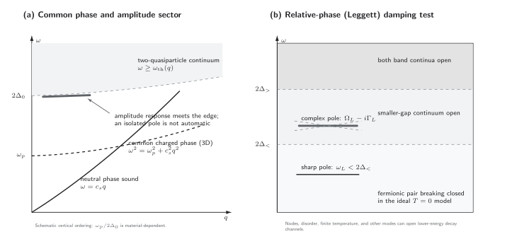
Pole and continuum structure for clean, fully gapped paired matter at zero temperature. The common-phase panel is schematic: the ordering of $\omega_p$ and $2\Delta_0$ is material-dependent. The relative-phase panel shows a kinematically protected example below $2\Delta_{<}$ and a complex-pole example after the smaller-gap continuum opens. Closure of the displayed fermionic channels does not guarantee probe weight, and an open channel broadens a pole only when its coupling is nonzero. Nodes, disorder, finite temperature, and other modes can open lower-energy decay channels. Original schematic, not to scale.

Download the SVG · Download the structured JSON equivalent

Diagnostics and justified conclusions

Candidate	Ideal kernel statement	Continuum and mixing test	Strongest justified conclusion
Neutral phase	$M_{\theta,\mathrm{eff}}(0,0)=0$ and $\omega=c_s q$	Verify the gap-equation cancellation, amplitude Schur complement, and positive $\chi_\theta,\rho_\theta$	Goldstone sound within the neutral low-energy theory
Common charged phase	A gauge-complete density–phase kernel gives the dimension-dependent plasma branch	Declare dimension, screening environment, electrodynamic regime, and conserving electromagnetic vertex	Gauge-invariant plasma response, not a missing phase degree of freedom
Amplitude response	The radial susceptibility is enhanced near $2\Delta_0$	Continue through the branch cut; retain amplitude–phase mixing and both probe vertices	Threshold feature unless an isolated amplitude-sector pole is demonstrated; nonzero residue is additionally required for visibility in the chosen probe
Leggett mode	The relative-phase determinant has a nonzero root	Use the full complex root near a continuum and test every coupled decay channel	Sharp if all coupled continua are closed, or every open-channel coupling vanishes; otherwise a width is allowed, and the full continuation decides whether a discernible resonance survives

The chapter-wide map places this kernel between the paired saddle and the responses that can observe it.

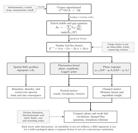
The shared paired-matter map locates collective modes in the larger inference chain. The page-local test is stricter: use one conserving approximation, continue the full determinant, identify the sheet and residue, and compare the root with every available continuum. Original schematic, not to scale.

The paired-matter claim test matrix summarizes the diagnostics and the conclusions they support.

Exercises

1. Recover the phase zero from the gap equation

Starting from the displayed trace, evaluate the fermionic Matsubara sum and show that $M_{\pi\pi}(0)=0$.

Solution

The standard sum is

$$T\sum_{\omega_n}\frac1{\omega_n^2+E^2} =\frac{1-2f(E)}{2E}.$$

Therefore

$$\Pi_{\pi\pi}(0) =-2\int_{\mathbf k}\frac{1-2f(E_{\mathbf k})}{2E_{\mathbf k}} =-\frac2g,$$

where the last step uses

$$\frac1g =\int_{\mathbf k}\frac{1-2f(E_{\mathbf k})}{2E_{\mathbf k}}$$

with the same ultraviolet prescription as the loop. Since $M_{\pi\pi}=2/g+\Pi_{\pi\pi}$, the terms cancel. A nonzero result obtained from different saddle and vertex approximations is a consistency failure, not a physical neutral phase gap.

2. Derive sound and the dimensional plasma laws

Let $\delta n$ be the pair-number density canonically conjugate to the pair phase $\theta$, let $\chi_n$ be its neutral compressibility in the same normalization, and let $q_*$ be the electric charge carried by one unit of $\delta n$. In Gaussian electrostatic units, take

$$\mathcal L =\delta n\,\dot\theta -\frac12\left[\chi_n^{-1}+V(q)\right](\delta n)^2 -\frac12\rho_\theta q^2\theta^2.$$

Integrate out $\delta n$. Find the neutral dispersion, then use $V_{\mathrm{3D}}(q)=4\pi q_*^2/(\epsilon q^2)$ and $V_{\mathrm{2D}}(q)=2\pi q_*^2/(\epsilon q)$ in the unscreened nonretarded regime.

Solution

The density equation is

$$\delta n=\frac{\dot\theta}{\chi_n^{-1}+V(q)}.$$

Substitution gives a phase kinetic coefficient $[\chi_n^{-1}+V(q)]^{-1}$, so

$$\omega^2(q) =\rho_\theta q^2\left[\chi_n^{-1}+V(q)\right].$$

For $V=0$, $\omega=c_s q$ with $c_s^2=\rho_\theta/\chi_n$. In three dimensions,

$$\omega^2(q) =\frac{4\pi\rho_\theta q_*^2}{\epsilon} +\frac{\rho_\theta}{\chi_n}q^2,$$

so the nonretarded mode has a nonzero $q=0$ plasma frequency. In an isolated two-dimensional layer,

$$\omega^2(q) =\frac{2\pi\rho_\theta q_*^2}{\epsilon}q +\frac{\rho_\theta}{\chi_n}q^2,$$

and therefore $\omega\propto\sqrt q$ over the unscreened electrostatic regime. Retardation or environmental screening changes the asymptotic law. Using constituent density instead of pair-number density requires translating the Berry term, compressibility, and charge together; mixing those conventions creates spurious factors of two or four.

3. Diagonalize and classify a two-band relative-phase root

Diagonalize the uniform diagonal two-phase action and find its eigenvectors and two frequencies. Then classify a proposed peak or root energy of $8\,\mathrm{meV}$ when $\Delta_1=3\,\mathrm{meV}$ and $\Delta_2=7\,\mathrm{meV}$.

Solution

For $\theta_a\propto e^{-i\omega t}$, the determinant is

$$\omega^2\left[ \chi_1\chi_2\omega^2-J(\chi_1+\chi_2) \right]=0.$$

The zero-frequency common-phase eigenvector is proportional to $(1,1)$. The relative eigenvector obeys

$$\chi_1\theta_1+\chi_2\theta_2=0,$$

so one convenient representative is $(\chi_2,-\chi_1)$. Its local-action frequency is

$$\omega_L^2 =J\left(\frac1{\chi_1}+\frac1{\chi_2}\right).$$

The ideal isotropic pair-breaking thresholds are $2\Delta_1=6\,\mathrm{meV}$ and $2\Delta_2=14\,\mathrm{meV}$. The proposed $8\,\mathrm{meV}$ feature lies above the first but below the second. Decay into band 1 is kinematically allowed if the coupling is nonzero. Because the local phase action is no longer reliable near the open continuum, the feature must be tested against the full frequency-dependent determinant and probe residue; it cannot yet be called an undamped eigenmode.

4. Distinguish a threshold singularity from a simple pole

Consider the toy retarded response

$$\chi_{\mathrm{th}}^R(\omega) =\frac{A}{ \sqrt{4\Delta_0^2-(\omega+i0^+)^2} }.$$

Show that $\omega=2\Delta_0$ is a branch point rather than a simple pole, even though the response is strongly enhanced there.

Solution

Near $\omega=2\Delta_0$, write $\omega=2\Delta_0+\delta$. Then

$$4\Delta_0^2-(\omega+i0^+)^2 =-4\Delta_0(\delta+i0^+)+O(\delta^2),$$

so $\chi_{\mathrm{th}}^R\propto(\delta+i0^+)^{-1/2}$. Analytic continuation around the threshold changes the sign of the square root, which identifies a two-sheeted branch point. By contrast, a simple pole would have a nonzero Laurent residue:

$$\lim_{\omega\to2\Delta_0} (\omega-2\Delta_0)\chi_{\mathrm{th}}^R(\omega).$$

Here that limit vanishes as $\sqrt{\delta}$. A broadened real-axis peak derived from this threshold may therefore be called a threshold enhancement, but not an amplitude-sector pole unless a separate isolated determinant zero exists away from the branch point. Nonzero residue is additionally required to see and attribute that pole in the chosen probe.

Continue

Superfluid order and phase stiffness defines the static pair-phase helicity modulus $\Upsilon$ with its source convention and order of limits; it should not be identified with $\rho_\theta$ here until those normalizations are matched. Gauge-invariant Meissner response then couples the charged system to electromagnetic probes and enforces the Ward and sum-rule checks behind screening and superfluid weight.

References

• Altland, A., and Simons, B. (2023). Condensed Matter Field Theory, 3rd ed. Cambridge University Press, ch. 6. doi:10.1017/9781108781244.
• Anderson, P. W. (1958). “Random-phase approximation in the theory of superconductivity.” Physical Review 112, 1900–1916. doi:10.1103/PhysRev.112.1900.
• Blumberg, G., Mialitsin, A., Dennis, B. S., Klein, M. V., Zhigadlo, N. D., and Karpinski, J. (2007). “Observation of Leggett’s collective mode in a multiband superconductor.” Physical Review Letters 99, 227002. doi:10.1103/PhysRevLett.99.227002.
• Cea, T., Castellani, C., Seibold, G., and Benfatto, L. (2015). “Nonrelativistic dynamics of the amplitude (Higgs) mode in superconductors.” Physical Review Letters 115, 157002. doi:10.1103/PhysRevLett.115.157002.
• Klein, M. V. (2010). “Theory of Raman scattering from Leggett’s collective mode in a multiband superconductor: Application to MgB$_2$.” Physical Review B 82, 014507. doi:10.1103/PhysRevB.82.014507.
• Leggett, A. J. (1966). “Number-phase fluctuations in two-band superconductors.” Progress of Theoretical Physics 36, 901–930. doi:10.1143/PTP.36.901.
• Littlewood, P. B., and Varma, C. M. (1982). “Amplitude collective modes in superconductors and their coupling to charge-density waves.” Physical Review B 26, 4883–4893. doi:10.1103/PhysRevB.26.4883.
• Nambu, Y. (1960). “Quasi-particles and gauge invariance in the theory of superconductivity.” Physical Review 117, 648–663. doi:10.1103/PhysRev.117.648.
• Pekker, D., and Varma, C. M. (2015). “Amplitude/Higgs modes in condensed matter physics.” Annual Review of Condensed Matter Physics 6, 269–297. doi:10.1146/annurev-conmatphys-031214-014350.
• Sharapov, S. G., Gusynin, V. P., and Beck, H. (2002). “Effective action approach to the Leggett’s mode in two-band superconductors.” European Physical Journal B 30, 45–51. doi:10.1140/epjb/e2002-00356-9.
• Stern, F. (1967). “Polarizability of a two-dimensional electron gas.” Physical Review Letters 18, 546–548. doi:10.1103/PhysRevLett.18.546.