Quantum-Matter Probes, Inference, and Evidence

Quantum-matter evidence begins with a recorded signal and ends with a conclusion whose strength is explicitly limited. Between them lie an operator, matrix element, kinematic map, background, resolution function, calibration, covariance, model, representation error, and alternative explanation. This chapter supplies that complete chain for major spectroscopies, local and cold-atom probes, QMC, tensor networks, exact diagonalization, model comparison, and reproducibility.

Helpful background. From measured intensity to many-body claim gives the common forward model. Transport extraction and inverse errors supplies the broader inverse-problem framework.

Evidence cutoff. This chapter covers primary and official sources checked through 10 August 2026. Later calibrations, platform records, replications, corrections, retractions, and changing assessments belong in the dated Quantum Matter and Emergence Research synthesis.

Enter this chapter

Start every analysis by writing the forward model

$$\text{record} =\text{background} +\text{resolution}\circ \text{matrix element}\circ \text{correlator} +\text{noise},$$

with state, geometry, units, and covariance declared. Then identify the strongest result actually needed: observation of a feature, assignment to an operator channel, parameter constraint, mechanism comparison, or phase inference. Each step requires a new test; none follows from visual prominence alone.

The first original figure gives the chapter’s common language. Follow its main horizontal path and notice that nuisance variables remain attached at every stage.

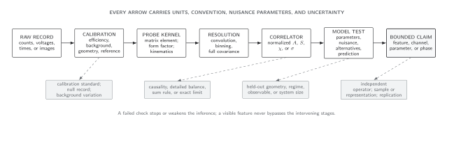
The measurement–correlator–claim dictionary. Every arrow is a documented transformation with propagated uncertainty; sum rules and negative controls can stop the inference before the final claim. Original schematic, not tied to one apparatus.

The route through the chapter is cumulative:

• From measured intensity to many-body claim defines forward kernels, normalization, covariance, and claim levels.
• ARPES maps photoelectron intensity to occupied one-particle spectral weight.
• STM and QPI distinguish local spectral density from impurity-mediated interference.
• Optical conductivity treats the electrodynamic inversion, causality, and spectral-weight sums.
• Neutron scattering maps kinematics and polarization to dynamical spin structure factors.
• Raman, RIXS, and EELS keep their distinct effective operators and resonance conditions.
• NMR and μSR connect local-spin precession and relaxation to field distributions and low-frequency response.
• Quantum oscillations infer extremal orbit areas, masses, damping, and conditional phases.
• Cold-atom probes treat RF, Bragg, expansion, in-situ imaging, and microscope detection.
• QMC phase inference propagates ensemble, sign, autocorrelation, scaling, and continuation limits.
• Tensor-network diagnostics propagate bond-dimension, geometry, optimization, and contraction limits.
• Exact diagonalization separates finite-matrix precision from thermodynamic inference.
• Model selection combines covariance, priors, nuisance parameters, discrepancy, and prediction.
• Evidence triangulation combines dependent evidence without counting shared assumptions twice.

Where evidence streams meet

The second original figure groups the experimental and computational branches. Their agreement is strongest when they test distinct operators or regimes and predict held-out results. Agreement inside one shared Hamiltonian, sample, calibration, or preprocessing pipeline is still useful, but it is not independent replication.

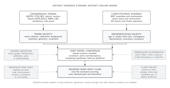
Evidence combination and failure map. Experimental resolution and calibration are not interchangeable with numerical finite-size and representation errors, and both branches can share a Hamiltonian or prior. Original schematic.

Probe and computation claim test matrix

Together with the preceding prose and figure alternatives, this table gives the nonvisual account of the two workflows. “Ceiling” is the strongest statement licensed before additional independent tests.

Route	Forward object	Main calibration or nuisance	Covariance or prior issue	Resolution or representation limit	Held-out or negative test	Claim ceiling
Measurement contract	Detector record from a convolved normalized correlator	Background, scale, geometry, efficiency	Shared calibration and processed-bin covariance	Singular directions of the response kernel	Reconstruct a reserved standard or synthetic truth	Calibrated observable or parameter constraint
ARPES	Dipole-weighted occupied $A(\mathbf k,\omega)$	Photon energy, polarization, surface, $k_z$	Background and global energy-reference covariance	Escape depth and energy–momentum resolution	Predict another polarization, photon energy, or termination	Dispersion or effective self-energy in a declared model
STM and QPI	Tip-weighted local spectrum and impurity response	Tip orbital, set point, surface, defect vertex	Drift correction and Fourier-window covariance	Thermal, voltage, spatial, and field-of-view limits	Reproduce several defects, fields, or terminations	Local gap or scattering geometry, not unique mechanism
Optical response	Fresnel or multilayer fields mapped to $\sigma(\omega)$	Thickness, tensor geometry, extrapolation	Kramers–Kronig and common-normalization covariance	Spectral window and low-frequency access	Recover causality and the applicable sum rule	Charge-dynamics scale or stiffness after missing-area checks
Neutron scattering	Polarization-projected $S^{\alpha\beta}(\mathbf Q,E)$	Form factor, absorption, monitor, mosaic	Shared background and four-dimensional resolution	Reciprocal-space coverage and resolution ellipsoid	Test equivalent zones, polarization, temperature, and sum rules	Mode or continuum in a stated spin channel
Raman, RIXS, EELS	Probe-specific effective response operator	Resonance, polarization, self-absorption, thickness	Normalization shared across incident energies or channels	Core-hole lifetime, screening, multiple scattering	Vary incident energy, symmetry channel, momentum, or thickness	Excitation assignment within a controlled operator reduction
NMR and μSR	Hyperfine- or site-weighted local-field correlations	Site, coupling tensor, dead time, background fraction	Correlated amplitudes and relaxation rates	Larmor and detector time window	Change nucleus or site sensitivity, field, and volume fraction	Static or dynamic local-field bound in a stated window
Quantum oscillations	Extremal orbit quantization	Angle, field background, temperature, torque geometry	Close-frequency and window covariance	Finite $1/B$ span, damping, magnetic breakdown	Predict angle, harmonic, thermodynamic, or transport response	Extremal area and mass; phase only with all corrections
Cold-atom probes	Expansion, transfer, response, or site-detection kernel	Trap, pulse, loss, Wannier envelope, detection matrix	Atom-number and image-processing covariance	Finite size, entropy, PSF, pulse and observation time	Benchmark a different observable, trap, preparation, or size	Realized correlator or finite-system phase evidence
Quantum Monte Carlo	Stochastic estimator in a declared representation	Ensemble, update, discretization, sign	Autocorrelation and cross-observable covariance	Size, temperature, Trotter or projection, continuation	Predict held-out sizes and exact limits; change formulation	Controlled equilibrium observable or scaled phase result
Tensor networks	Variational state and transfer environment	Initialization, unit cell, symmetry, geometry	Correlated extrapolations and ansatz selection	Bond dimension, cylinder width, contraction dimension	Competing states, boundaries, bond dimensions, observables	Variational phase evidence after representation scaling
Exact diagonalization	Eigenpairs and dynamics of a finite sector	Symmetry, cluster, boundary, broadening	Disorder-sample and spectral-window covariance	Exponential size limit and recurrences	Hold out cluster shapes, twists, and sizes	Exact finite-system result with bounded extrapolation
Model selection	Joint generative likelihood	Nuisance parameters and discrepancy	Full covariance and prior-volume sensitivity	Candidate-set and emulator limits	Leave out a probe, regime, or defining observable	Relative predictive support, not unique truth
Triangulation	Dependence graph of evidence and claims	Versions, samples, shared Hamiltonian, preprocessing	Shared ancestors prevent naive likelihood products	Reproduction and replication scope	Independent data, representation, perturbation, and null tests	Conclusion surviving distinct failure modes

Five rules for strong inference

1. Fit the rawest defensible observable with the forward kernel; do not deconvolve away uncertainty.
2. Carry units, normalization, covariance, and nuisance parameters through every transformation.
3. Test exact limits, detailed balance, Ward identities, or sum rules before interpreting features.
4. Compare a physically plausible alternative and reserve a prediction that was not used in model construction.
5. State the conclusion at the weakest untested link: finite window, finite size, representation, surface, calibration, or candidate set.

These rules combine the measurement-equation discipline of Possolo 2015, probe-specific standards exemplified by Sobota, He, and Shen 2021 and Bloch, Dalibard, and Zwerger 2008, predictive comparison diagnostics from Vehtari, Gelman, and Gabry 2017, and reproducibility principles from Wilkinson et al. 2016 and the National Academies 2019.

A reproducible verification should include synthetic convolution, covariance-aware model comparison, and adversarial false-positive tests. The pages and semantic table provide the complete noninteractive treatment.

Review the chapter

1. Rank two agreements. ARPES and STM on one cleave agree on a gap scale, while neutron scattering on a separately prepared crystal predicts and observes the momentum of a collective mode using parameters fixed elsewhere. Which is more independent evidence, and why?

Solution

ARPES and STM use different one-particle matrix elements, so their agreement is valuable, but they share a surface, sample preparation, and possibly the same gap model. The neutron result uses a different operator, specimen, and held-out momentum prediction, so it normally contributes more independent mechanism evidence—provided the samples occupy the same phase and the prediction was genuinely fixed in advance.

2. Stop a phase claim. A sign-free QMC crossing and a tensor-network low-energy state agree on a finite cylinder, but both use the same effective Hamiltonian and neither predicts an available experimental polarization channel. What is the strongest conclusion?

Solution

The two methods provide cross-representation evidence for the finite-size behavior of the shared Hamiltonian. The conclusion should stop before material realization or a unique phase mechanism until size and representation limits are stable, competing phases are tested, and the held-out experimental channel is predicted successfully. Their shared Hamiltonian is a common assumption, not independent evidence for that assumption.

References

• Immanuel Bloch, Jean Dalibard, and Wilhelm Zwerger, “Many-Body Physics with Ultracold Gases,” Reviews of Modern Physics 80 (2008) 885–964. DOI
• National Academies of Sciences, Engineering, and Medicine, Reproducibility and Replicability in Science, National Academies Press, 2019. DOI
• Antonio Possolo, Simple Guide for Evaluating and Expressing the Uncertainty of NIST Measurement Results, NIST Technical Note 1900, 2015. DOI
• Jonathan A. Sobota, Yu He, and Zhi-Xun Shen, “Angle-Resolved Photoemission Studies of Quantum Materials,” Reviews of Modern Physics 93 (2021) 025006. DOI
• Aki Vehtari, Andrew Gelman, and Jonah Gabry, “Practical Bayesian Model Evaluation Using Leave-One-Out Cross-Validation and WAIC,” Statistics and Computing 27 (2017) 1413–1432. DOI
• Mark D. Wilkinson, Michel Dumontier, IJsbrand Jan Aalbersberg, Gabrielle Appleton, Myles Axton, Arie Baak, Niklas Blomberg, Jan-Willem Boiten, Luiz Bonino da Silva Santos, Philip E. Bourne, Jildau Bouwman, Anthony J. Brookes, Tim Clark, Mercè Crosas, Ingrid Dillo, Olivier Dumon, Scott Edmunds, Chris T. Evelo, Richard Finkers, Alejandra Gonzalez-Beltran, Alasdair J. G. Gray, Paul Groth, Carole Goble, Jeffrey S. Grethe, Jaap Heringa, Peter A. C. ’t Hoen, Rob Hooft, Tobias Kuhn, Ruben Kok, Joost Kok, Scott J. Lusher, Maryann E. Martone, Albert Mons, Abel L. Packer, Bengt Persson, Philippe Rocca-Serra, Marco Roos, Rene van Schaik, Susanna-Assunta Sansone, Erik Schultes, Thierry Sengstag, Ted Slater, George Strawn, Morris A. Swertz, Mark Thompson, Johan van der Lei, Erik van Mulligen, Jan Velterop, Andra Waagmeester, Peter Wittenburg, Katherine Wolstencroft, Jun Zhao, and Barend Mons, “The FAIR Guiding Principles for Scientific Data Management and Stewardship,” Scientific Data 3 (2016) 160018. DOI