Doped Mott Matter and the Pseudogap Evidence Problem

A pseudogap claim contains three different questions: is low-energy spectral weight suppressed, where does that crossover occur, and what causes it? In specified regimes of the two-dimensional Hubbard model, a momentum-selective pseudogap now has strong support from complementary calculations and a momentum-sensitive quantum-simulator experiment, while a separate microscope experiment supplies cross-observable magnetic-correlation evidence. That operational result does not by itself choose a unique mechanism for every parameter set or for real cuprates.

Required background. Use spectral-weight transfer and cluster-DMFT validity. Helpful background. Competing orders and ARPES inference supply key alternatives and probe effects.

Coordinates of a pseudogap claim

For the one-band square-lattice model, state the hopping ratios, interaction $U/t$, temperature $T/t$, lattice size or thermodynamic-limit procedure, and allowed symmetries. We define the filling $n$ per site and signed doping

$$\delta=1-n,$$

so $\delta>0$ is hole doping and $\delta<0$ is electron doping. A comparison that changes $t'/t$, constrains a normal state, or permits superconducting, magnetic, charge, or nematic order has changed the scientific question.

In a spin-rotation-invariant state, suppressing the spin label, use the per-spin spectral function

$$\begin{aligned} A_\sigma(\mathbf k,\omega) &=-2\operatorname{Im}G^R_\sigma(\mathbf k,\omega),\\ \int_{-\infty}^{\infty}\frac{\mathrm d\omega}{2\pi} A_\sigma(\mathbf k,\omega)&=1. \end{aligned}$$

Below, $A$ and $G$ denote these per-spin quantities; a spin-summed spectral function has zeroth moment $2$.

A spectral pseudogap is a reproducible suppression around $\omega=0$ relative to neighboring frequencies and a declared high-temperature or doping baseline. It is not a complete charge gap: a doped pseudogap metal can remain compressible, whereas a charge insulator has vanishing zero-temperature compressibility

$$\kappa=\left.\frac{\partial n}{\partial\mu}\right|_T$$

in the thermodynamic limit, with thermally activated corrections at $T>0$.

On a cuprate-like Fermi contour, the nodal sector lies near the zone diagonal and $(\pi/2,\pi/2)$; the antinodal sector lies near $(\pi,0)$ and symmetry-related points. These names are geometric. Suppressing antinodal weight while retaining nodal weight establishes momentum differentiation, not $d$-wave pairing. A thresholded intensity map can show apparent “arcs,” but it does not prove that the underlying Fermi contour is literally open.

The figure shows the distinction to inspect: the reference contour can remain closed even though a low-intensity threshold retains only nodal segments, while the antinodal line shape develops a central depression.

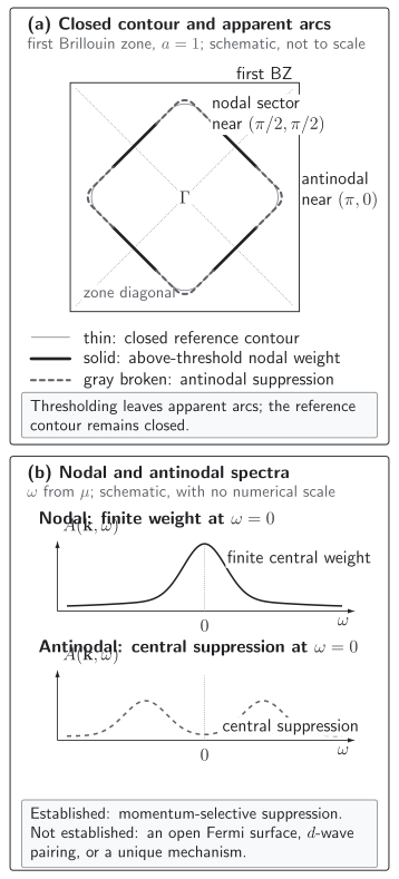
Momentum-selective pseudogap and apparent arcs. The thin gray line is one closed schematic reference contour; solid dark nodal segments remain above a low-energy intensity threshold, while broken gray antinodal segments mark suppressed weight on that same contour. The accompanying line shapes retain nodal weight at $\omega=0$ but suppress antinodal weight. This schematic, not-to-scale comparison establishes neither pairing nor a unique microscopic mechanism.

Open the figure at full size or download its semantic JSON.

Keep three scales distinct:

• a pseudogap energy $\Delta_{\mathrm{pg}}$ extracted under a declared line-shape model;
• an onset crossover $T_A^*$ for a spectral diagnostic; and
• an endpoint doping $\delta^*$ under fixed Hamiltonian and symmetry conditions.

A spin-response crossover may define $T_\chi^*$. A maximum of $\kappa(T)$ at fixed $\delta$ can define $T_\kappa^*(\delta)$, whereas a maximum of $\kappa(\delta)$ at fixed $T$ defines a doping coordinate $\delta_\kappa^*(T)$, not a temperature. There is no reason for all of these broad finite-temperature markers to coincide.

Diagnostics before and after analytic continuation

The thermal-window estimator

Imaginary-time data provide a continuation-free low-energy diagnostic. The spectral representation at $\tau=\beta/2$ is

$$-G(\mathbf k,\beta/2) =\int_{-\infty}^{\infty}\frac{\mathrm d\omega}{2\pi}\, \frac{A(\mathbf k,\omega)}{2\cosh(\beta\omega/2)}.$$

The kernel is even, centered at zero frequency, and has width of order $T$. More precisely,

$$K_\beta(\omega) =\frac{\beta}{2\pi\cosh(\beta\omega/2)}, \qquad \int_{-\infty}^{\infty}\mathrm d\omega\,K_\beta(\omega)=1,$$

so the exact estimator is the thermal average

$$\widetilde A_\beta(\mathbf k,0) \equiv-2\beta G(\mathbf k,\beta/2) =\int_{-\infty}^{\infty}\mathrm d\omega\, K_\beta(\omega)A(\mathbf k,\omega).$$

If $A(\mathbf k,\omega)$ is smooth across that window, then $\widetilde A_\beta(\mathbf k,0)\approx A(\mathbf k,0)$. The estimator avoids an inversion, but it cannot resolve features narrower than the thermal window or determine a sharp gap edge. An equivalent $\beta/2$ diagnostic, written with the conventional unit-normalized spectral function, is used by Malcolms et al. 2026, “Fermi surfaces, Fermi arcs, and spectral functions,” equation following Fig. 1 and Fig. 2.

Analytic continuation and Green-function zeros

Analytic continuation reconstructs real-frequency information from discrete, noisy imaginary-time data. This inverse problem is ill-conditioned: distinct spectra can fit the same data within uncertainty. Continued spectra therefore offer more detail while inheriting the prior, covariance model, frequency grid, and resolution of the continuation. A strong claim should show both the imaginary-axis evidence and the continuation sensitivity.

The relation

$$G^{-1}(\mathbf k,z) =z+\mu-\epsilon_{\mathbf k}-\Sigma(\mathbf k,z)$$

also clarifies claims about zeros. A true zero of $G$ requires an appropriate self-energy divergence in a controlled limiting procedure. A finite-depth spectral depression at nonzero temperature is not automatically a zero. In a cluster calculation, any lattice zero surface reconstructed from cluster data should be tested against cluster size and reconstruction choices. A cumulant-periodized CDMFT plus exact-diagonalization calculation illustrates how poles and zeros can organize a spectrum Sakai, Motome, and Imada 2009, Eq. (2) and Figs. 1–2, but a self-energy pole or successful gauge-theory interpretation does not by itself establish fractionalization Wu et al. 2018, abstract, § III.E, and § V.

Triangulating related crossovers

Different probes weight different correlators. Their agreement is powerful only after their nuisance parameters are exposed.

Quantity or probe	Operational signal	Principal controls	Strongest direct inference
$A(\mathbf k,\omega)$ from a calculation	central suppression relative to a fixed baseline; nodal–antinodal contrast	cluster and size drift, frequency resolution, continuation covariance, spectral sum rule	momentum-resolved spectral pseudogap in the declared model
$-2\beta G(\mathbf k,\beta/2)$	stable loss of thermally averaged low-energy weight	finite-$T$ kernel, statistics, momentum resolution	continuation-free corroboration over an $O(T)$ window
ARPES intensity	leading-edge or line-shape suppression with momentum dependence	matrix elements, Fermi factor, background, surface, energy and momentum resolution	material surface spectral suppression, not directly $A$ or a mechanism
Local tunneling spectrum	depression of low-bias differential conductance	tunneling matrix element, set point, disorder, surface, momentum integration	local weighted density-of-states suppression
Knight shift or uniform $\chi_s$	maximum or decrease after orbital subtraction	hyperfine coupling, orbital contribution, field, material calibration	crossover in the uniform spin response
$1/T_1T$ or low-frequency spin response	change in a hyperfine-weighted momentum sum	form factor, low-frequency limit, competing magnetic order	redistribution of slow spin fluctuations
Compressibility $\kappa$	maximum versus doping or temperature, or low-$T$ suppression	equation-of-state derivative, trap or finite-size effects, thermometry	thermodynamic crossover; not by itself a spectral gap
Entropy or heat capacity	anomaly, inflection, or redistribution across a declared baseline	subtraction, integration constants, phonons, finite-size effects	thermodynamic reorganization, not a unique single-particle scale
Lattice-modulation spectroscopy	loss of low-frequency response in a calibrated kernel	drive response, trap averaging, heating, calibration	simulator response consistent with a pseudogap; not ARPES

For nuclear magnetic resonance (NMR), the Knight shift mainly probes the uniform static response. With spin isotropy and omitted calibration constants, relaxation probes fluctuations transverse to the nuclear quantization axis:

$$\frac1{T_1T}\propto \sum_{\mathbf q}\lvert F_{\mathrm{hf}}(\mathbf q)\rvert^2 \lim_{\omega\to0} \frac{\operatorname{Im}\chi^{+-}(\mathbf q,\omega)}{\omega},$$

where $F_{\mathrm{hf}}$ is the hyperfine form factor Wang et al. 2026, Appendix A.4, Eqs. (A28)–(A36). The two quantities need not turn over at the same temperature. Likewise, a maximum in $\kappa(\delta)$ is a crossover marker, not evidence that the metal has become incompressible Vilk and Tremblay 2026, §§ III–VI and Figs. 1–7.

What the Hubbard-model evidence now supports

Evidence cutoff: 31 August 2026. Last substantive scientific update: 31 August 2026. The assessment table and model-specific evidence below use a finite set of primary results chosen for complementary control, direct bearing on the square-lattice pseudogap, and explicit limitations. A version of record supersedes its preprint here; related papers using the same data or approximation are not counted as independent replications.

Widom-line organization

One proposed organizing line needs an operational definition. In the constrained normal-state $2\times2$ plaquette cellular dynamical mean-field theory (CDMFT) construction of Sordi et al., long-range magnetic, superconducting, and other broken-symmetry states are not admitted. Within that construction, the Widom line continues above a finite-doping first-order critical endpoint as the locus where maxima of different response functions converge. They estimate it from maxima, as the chemical potential is varied, of their physical-compressibility convention $\kappa_T=n^{-2}(\partial n/\partial\mu)_T$. The factor $n^{-2}$ is not constant on a doping scan, so these extrema need not coincide with maxima of the charge susceptibility $\kappa=(\partial n/\partial\mu)_T$ defined above; indeed an interior stationary point of $\kappa_T(\mu)$ obeys $\mathrm d\kappa/\mathrm d\mu=2\kappa^2/n$, not $\mathrm d\kappa/\mathrm d\mu=0$. Compare locations only after matching conventions. Spectral and spin crossover lines approach the Widom locus in the same construction Sordi et al. 2012, Figs. 1–4 and Methods. This is a model- and cluster-specific organization, not a universal property of every pseudogap calculation.

Cross-method consensus

Claim	Assessment at the cutoff	Evidence ceiling
An operational pseudogap occurs in specified two-dimensional Hubbard regimes	Strong multi-method support. Cluster methods, thermodynamic-limit diagrammatic Monte Carlo, determinant QMC, and one momentum-sensitive quantum-simulator experiment find low-energy suppression in complementary, partly overlapping but nonidentical Hamiltonians and temperature windows; a separate simulator observes correlated magnetic scaling in the same model.	Not every $U/t$, $t'/t$, doping, temperature, or enforced symmetry sector is covered. The second simulator is cross-observable support, not an independent spectral measurement.
The suppression is momentum selective	Strong support. Antinodal weight is depleted before nodal weight in several calculations and in momentum-sensitive simulator response.	Sector resolution, continuation, and reconstruction remain method dependent.
Spin correlations dominate the nearest-neighbor model’s nonlocal pseudogap scattering	Strong, parameter-bounded support. Controlled diagrammatic calculations reproduce the nonlocal self-energy quantitatively with a modified spin-fluctuation form at weak coupling and qualitatively at strong coupling. An independent quantum-gas-microscope experiment finds a magnetic scaling scale consistent with a numerically defined uniform-susceptibility crossover.	The microscope result is cross-observable consistency, not an independent spectral measurement or causal intervention. At strong coupling, one fitted vertex does not reproduce both real and imaginary self-energy, the large local part lies outside that ansatz, and the short correlation length invalidates a conventional long-range spin-density-wave picture.
The finite-temperature pseudogap extrapolates to the stripe-ordered ground-state domain	Consistent with one controlled extrapolation, not established as a unique continuation. The extrapolated finite-temperature boundary agrees within reported uncertainty with a separately calculated ground-state stripe boundary.	The continuation is not observed directly; extrapolation form, ground-state method, and stripe commensurability remain relevant.
All probes share one $T^*$	Not supported. Spectral, NMR-like, compressibility, and correlation crossovers can differ.	A shared scale requires a quantitative mapping of response kernels and uncertainties.
A Widom line or a Green-function-zero surface uniquely organizes the pseudogap	Method-supported, not unique. Both can organize particular calculations.	Their location and even visibility can depend on reconstruction, observable, and model.
The one-band result fixes the mechanism of the cuprate pseudogap	Open.	Cuprates are charge-transfer, multiorbital materials with further-neighbor hopping, phonons, disorder, longer-range interactions, and intertwined orders.

Several results materially set this assessment. Cluster calculations establish a normal-state pseudogap within a declared finite-cluster construction and expose its competition with superconductivity Gull, Parcollet, and Millis 2013, Figs. 1–2. Thermodynamic-limit diagrammatic Monte Carlo finds antinodal destruction at low doping at both weak and strong coupling, reproduces the nonlocal self-energy quantitatively with a modified spin-fluctuation form at weak coupling but only qualitatively at strong coupling, and extrapolates the finite-temperature boundary to a separately calculated stripe-ordered ground-state domain Šimkovic et al. 2024, Figs. 1 and 3–5. Ultracold-atom measurements combine a compressibility maximum with symmetry-sensitive lattice-modulation spectra and map an underdoped pseudogap regime; this operational evidence does not by itself identify a magnetic cause, and the authors instead discuss a possible connection to incipient charge order Kendrick et al. 2026, Figs. 2–4. On an independent quantum-gas-microscope platform, multipoint spin–charge correlations yield a spin-stiffness-like scale $\Delta(\delta)$ comparable to—but slightly below—the uniform-susceptibility crossover $T_\chi^*$ obtained from minimally entangled typical thermal states. The authors do not establish a formal equality, so this is cross-observable consistency rather than an independent spectral-pseudogap measurement Chalopin et al. 2026, Fig. 3 and discussion.

Probe-indexed crossover scales

The newest version-of-record results strengthen the need for probe-indexed crossovers. The two-particle self-consistent plus method (TPSC+) relates the compressibility maximum to an antinodal spin-density-wave precursor crossing and separately predicts doping- and temperature-dependent Knight-shift maxima within its weak- and intermediate-coupling domain Vilk and Tremblay 2026, abstract and Figs. 1–7. At $U/t=6$ and $t'/t=-0.25$ on mainly $8\times8$ lattices, with $t''$ and size checks, high-resolution determinant quantum Monte Carlo (DQMC) finds electron–hole asymmetry and a low-doping nodal–antinodal dichotomy. It attributes the hole-doped suppression in that parameter set to the momentum-dependent remnant Mott gap rather than to control by the short magnetic correlation length, while its simulated NMR and spectroscopic crossover temperatures need not agree Wang et al. 2026, Figs. 7 and 11–14, Appendix A.4, and Appendices B–C. As developed in the QMC inference protocol, doping introduces a sign problem and the spectra additionally retain size, temperature, twist-grid, and continuation limits. TPSC+ is an approximate weak- to intermediate-coupling framework, while the successful real-frequency calculation of Geng et al. uses a one-shot TPSC+DMFT construction with a noncrossing-approximation impurity solver; the tested self-consistent variants underestimate nonlocal correlations and miss the pseudogap. Neither method is an exact solver Geng, Yan, and Werner 2025, §§ II.C–D and III–IV.

Mechanism tests, not mechanism labels

Candidate explanation	Evidence that would discriminate it	What the same pseudogap data do not establish
Short-range antiferromagnetic or spin-density-wave fluctuations	quantitative covariance of spin correlations and the momentum-dependent self-energy; intervention by changing correlation length; agreement across controlled methods	a universal weak-coupling hot-spot picture or direct transfer to every cuprate
Mott proximity, thermodynamic crossover, or Green-function zeros	stable pole/zero structure across cluster families and reconstructions; thermodynamic inflections tied to the same parameter line	fractionalization, a unique Widom line, or a zero-temperature phase
Precursor pairing	enhanced pairing susceptibility and pair correlations above $T_c$, with a gap scale that follows them when other orders are controlled	that any antinodal suppression is pairing, or that pairing is necessary for the normal-state Hubbard pseudogap
Stripe, charge, or nematic order	size-stable structure factors, symmetry breaking, correlation lengths, and an onset ordered relative to the spectral crossover	causation merely because order appears nearby or at lower temperature
Fractionalized Fermi liquid or resonating-valence-bond (RVB) physics	fractionalization-specific response, topological structure, gauge-sector signatures, and a controlled modified-volume relation	a fractionalized state from Fermi arcs, a self-energy pole, or anomalous transport alone
Band structure, van Hove physics, disorder, or probe effects	a matched noninteracting baseline, $t'$ and material dependence, disorder scaling, and matrix-element or resolution controls	that every loss of measured intensity is an interaction-driven pseudogap

The chapter validity map and semantic table encode the same observation-versus-mechanism ceiling. An operational pseudogap may remain well established while several causal descriptions remain live.

From a Hubbard model to a cuprate claim

The one-band Hubbard model isolates an important mechanism question, but a cuprate parent is a charge-transfer insulator with copper and oxygen orbitals. At a fixed Emery-model parameterization and temperatures of roughly $251$–$377\,\mathrm K$, a three-band ladder dynamical vertex approximation (ladder DΓA) calculation also finds nodal–antinodal differentiation and attributes the normal-state pseudogap in that domain to short-range antiferromagnetic fluctuations Malcolms et al. 2026, Figs. 2–4 and Methods. This narrows the model-transfer gap; it does not remove approximation error or establish a universal material mechanism.

Real materials add superconducting fluctuations, charge and nematic order, phonons, disorder, surfaces, long-range Coulomb interactions, and probe matrix elements. For a synthesis of the resulting robust cuprate phenomenology and its unresolved causal hierarchy, see the review by Keimer et al. 2015, pp. 179–186. For the wider dated research context, use Quantum Matter and Emergence; this page retains the narrower Hubbard-to-cuprate evidence boundary.

Common pitfalls

Calling every depression a gap. A pseudogap needs a baseline, uncertainty, and stable low-energy suppression. Broadening, a van Hove feature, a matrix-element node, or insufficient thermal resolution can mimic one.

Treating an arc as an open Fermi surface. An arc is usually a thresholded locus of low-energy intensity. Its invisible side may be broadened or weak rather than absent.

Turning a crossover into a phase boundary. A maximum or inflection can be an excellent operational marker without a singular free energy. Name the observable that defines each $T^*$.

Inferring one mechanism from several correlated observables. Triangulation strengthens the observation. Mechanism attribution additionally requires interventions or discriminants that separate live alternatives.

Exercises

1. Normalize the thermal-window estimator

Derive the $\beta/2$ estimator when $A(\mathbf k,\omega)$ is approximately constant over the thermal kernel.

Solution

Set $A(\mathbf k,\omega)\approx A(\mathbf k,0)$ in the spectral representation. With $x=\beta\omega/2$,

$$\int_{-\infty}^{\infty} \frac{\mathrm d\omega}{2\cosh(\beta\omega/2)} =\frac{\pi}{\beta}.$$

Hence $-G(\mathbf k,\beta/2)\approx A(\mathbf k,0)/(2\beta)$ and $-2\beta G(\mathbf k,\beta/2)\approx A(\mathbf k,0)$. Because the kernel is even in $\omega$, the odd part of the spectral asymmetry cancels. The approximation fails when the even part varies appreciably across the $O(T)$ window or when it contains structure narrower than that window.

2. Separate continuation from imaginary-time evidence

A continued cluster spectrum shows suppressed antinodal $A(\mathbf k,0)$, but the continuation-free estimator $-2\beta G(\mathbf k,\beta/2)$ remains consistent with its declared high-temperature baseline within error at both cluster sizes. What is the strongest conclusion?

Solution

The finite-cluster continuation suggests an antinodal suppression, but there is no imaginary-axis corroboration and its thermodynamic robustness is not established. One should report the continuation- and cluster-dependent tendency, examine covariance, and, where the cluster construction requires periodization or another lattice reconstruction, vary that choice. Avoid a phase or mechanism claim until a size-stable observable shows baseline-relative suppression.

3. Keep crossover temperatures probe indexed

Spectroscopy gives $T_A^*=0.20t$, while an NMR-like uniform-spin diagnostic turns over at $T_\chi^*=0.14t$. Is one result necessarily wrong?

Solution

No. The probes integrate different momenta and frequencies and can respond to different stages of a broad crossover. First verify thermometry, response kernels, finite-size drift, and uncertainties. If both survive, report two probe-indexed crossover temperatures rather than forcing a unique $T^*$.

4. Test a claimed Green-function zero

A periodized calculation has $A(\mathbf k,0)>0$ but a deep minimum and a rapidly growing self-energy. Has it demonstrated a Green-function zero?

Solution

No. For the reported broadened finite-temperature object, $A(\mathbf k,0)=-2\operatorname{Im}G^R(\mathbf k,0)>0$ directly excludes an exact zero of $G^R$ at that point. A putative zero of an underlying limiting function requires controlled $\eta\to0^+$, $T\to0$, and cluster or thermodynamic extrapolations with their order stated; where periodization is used, it must survive that choice as well. Even then, the zero would not by itself establish fractionalization.

5. Distinguish covariance from causation

A quantum simulator, diagrammatic Monte Carlo, and cluster DMFT all find an antinodal pseudogap in closely related Hubbard regimes, and spin correlations track its onset. No channel-resolved self-energy decomposition or controlled intervention is supplied. State the strongest bounded inference.

Solution

The stated evidence establishes a robust momentum-selective pseudogap whose onset covaries with spin correlations across the declared parameter and temperature windows. Those facts alone do not establish magnetic causation. That stronger conclusion requires a channel-resolved self-energy test or an intervention that distinguishes spin physics from Mott proximity and other live alternatives; neither would by itself fix the mechanism of every cuprate.

References

• Thomas Chalopin, Petar Bojović, Si Wang, Titus Franz, Aritra Sinha, Zhenjiu Wang, Dominik Bourgund, Johannes Obermeyer, Fabian Grusdt, Annabelle Bohrdt, Lode Pollet, Alexander Wietek, Antoine Georges, Timon Hilker, and Immanuel Bloch, “Observation of Emergent Scaling of Spin–Charge Correlations at the Onset of the Pseudogap,” Proceedings of the National Academy of Sciences 123 (2026) e2525539123, doi:10.1073/pnas.2525539123.
• Lei Geng, Jiawei Yan, and Philipp Werner, “Two-Particle Self-Consistent Approach Combined with Dynamical Mean Field Theory: A Real-Frequency Study of the Square-Lattice Hubbard Model,” Physical Review B 111 (2025) 115143, doi:10.1103/PhysRevB.111.115143.
• Emanuel Gull, Olivier Parcollet, and Andrew J. Millis, “Superconductivity and the Pseudogap in the Two-Dimensional Hubbard Model,” Physical Review Letters 110 (2013) 216405, doi:10.1103/PhysRevLett.110.216405, Open PDF.
• Bernhard Keimer, Steven A. Kivelson, Michael R. Norman, Shin-ichi Uchida, and Jan Zaanen, “From Quantum Matter to High-Temperature Superconductivity in Copper Oxides,” Nature 518 (2015) 179–186, doi:10.1038/nature14165.
• Lev Haldar Kendrick, Anant Kale, Youqi Gang, Alexander Dennisovich Deters, Martin Lebrat, Aaron W. Young, and Markus Greiner, “Pseudogap in a Fermi–Hubbard Quantum Simulator,” Nature 656 (2026) 602–608, doi:10.1038/s41586-026-10875-z, data and code.
• M. O. Malcolms, Henri Menke, Yi-Ting Tseng, Eric Jacob, Karsten Held, Philipp Hansmann, and Thomas Schäfer, “Rise and Fall of the Pseudogap in the Emery Model, Insights for Cuprates,” Communications Physics 9 (2026) 179, doi:10.1038/s42005-026-02685-6.
• Shiro Sakai, Yukitoshi Motome, and Masatoshi Imada, “Evolution of Electronic Structure of Doped Mott Insulators: Reconstruction of Poles and Zeros of Green’s Function,” Physical Review Letters 102 (2009) 056404, doi:10.1103/PhysRevLett.102.056404.
• Fedor Šimkovic IV, Riccardo Rossi, Antoine Georges, and Michel Ferrero, “Origin and Fate of the Pseudogap in the Doped Hubbard Model,” Science 385 (2024) eade9194, doi:10.1126/science.ade9194.
• Giovanni Sordi, Patrick Sémon, Kristjan Haule, and A.-M. S. Tremblay, “Pseudogap Temperature as a Widom Line in Doped Mott Insulators,” Scientific Reports 2 (2012) 547, doi:10.1038/srep00547.
• Y. M. Vilk and A.-M. S. Tremblay, “Pseudogap, Fermi Liquid, Van Hove Singularity, and Maxima of the Compressibility and of the Knight Shift as a Function of Doping in the Two-Dimensional Hubbard Model,” Physical Review X 16 (2026) 031034, doi:10.1103/7v3y-tbbr.
• Wen O. Wang, Edwin W. Huang, Brian Moritz, and Thomas P. Devereaux, “Probing the Pseudogap and Beyond: Examining Single-Particle Properties of the Hole- and Electron-Doped Hubbard Model,” Physical Review B 114 (2026) 105126, doi:10.1103/mqz8-h38p.
• Wei Wu, Mathias S. Scheurer, Shubhayu Chatterjee, Subir Sachdev, Antoine Georges, and Michel Ferrero, “Pseudogap and Fermi-Surface Topology in the Two-Dimensional Hubbard Model,” Physical Review X 8 (2018) 021048, doi:10.1103/PhysRevX.8.021048.