DMFT Impurity Mapping and Self-Consistency

Dynamical mean-field theory (DMFT) replaces the local environment of a lattice site by a quantum impurity in a bath that the lattice itself determines. For a Hubbard model on the standard large-dimensional or large-connectivity lattice sequences, scaling nearest-neighbor hopping as $t_{ij}=O(\mathcal Z^{-1/2})$ keeps the kinetic scale finite and makes the irreducible one-particle self-energy local while preserving its full frequency dependence. DMFT is therefore a controlled infinite-coordination mapping—not a generic large-$U$ approximation. In finite dimension, the same equations define the single-site-DMFT approximation and require an independent test of neglected spatial correlations.

Required background. Use the Hubbard model and its limits. Helpful background. Conserving self-energy constructions and quantum impurity models provide useful context.

We use the kinetic convention $H_t=-\sum_{ij\sigma}t_{ij}c_{i\sigma}^\dagger c_{j\sigma}$ and the thermal Green function

$$G_{ij,\sigma}(\tau) =-\langle \mathrm T_\tau c_{i\sigma}(\tau)c_{j\sigma}^\dagger(0)\rangle.$$

Here $z$ denotes either a Matsubara frequency $i\omega_n$ or a retarded argument $\omega+i0^+$, as appropriate. The superscript in the cavity propagator $G_{ij}^{(0)}$ means “site $0$ removed”; the calligraphic Weiss propagator $\mathcal G_0$ describes the noninteracting impurity bath. They are related by the construction below but are not the same object.

Why locality makes an impurity possible

The finite-second-moment condition

$$\sum_j\lvert t_{ij}\rvert^2=O(1)$$

fixes the kinetic scale; nearest-neighbor hopping $t^*/\sqrt{\mathcal Z}$ is one realization Metzner and Vollhardt 1989, printed p. 324, eq. (3). On the standard large-$d$ or large-$\mathcal Z$ sequences for which the usual path and diagram power counting applies, nonlocal self-energy contributions vanish for a local interaction:

$$\Sigma_{ij,\sigma}(z)=\delta_{ij}\Sigma_{i,\sigma}(z).$$

In a homogeneous normal state, $\Sigma_{i,\sigma}$ is site independent, and it is spin independent in the paramagnet. The second-moment condition alone is not a locality theorem for an arbitrary high-degree graph. Locality also does not mean static mean field: $\Sigma(z)$ retains all local quantum dynamics Georges et al. 1996, § II.A, printed p. 18, eqs. (12)–(13), and § III.B, printed pp. 23–24, eqs. (39)–(43). If translation symmetry is broken, the limiting self-energy remains site-local but can differ between sublattices and spin sectors Georges et al. 1996, § V, printed pp. 31–32.

Choose site $0$ and remove it temporarily. Let $G_{ij}^{(0)}$ be the interacting Green function of this cavity lattice. In the controlled large-coordination limit, the cavity and full Green functions obey

$$G_{ij}^{(0)}(z) =G_{ij}(z)-\frac{G_{i0}(z)G_{0j}(z)}{G_{00}(z)}, \qquad i,j\ne0.$$

This relation becomes exact in that limit; it is not an ordinary finite-dimensional matrix identity for an interacting system whose environment changes when a site is removed. Hopping from site $0$ into the cavity and back produces the hybridization

$$\Delta_0(z)=\sum_{i,j\ne0}t_{0i}\,G_{ij}^{(0)}(z)\,t_{j0}.$$

Connected cavity cumulants beyond quadratic order vanish under the same power counting. The environment of site $0$ is consequently a Gaussian fermionic bath. Its bath-dressed, locally noninteracting propagator is

$$\mathcal G_0^{-1}(z)=z+\mu-\Delta_0(z).$$

The surviving local interaction gives the impurity action

$$\begin{aligned} S_{\mathrm{imp}} ={}&-\sum_\sigma\int_0^\beta\mathrm d\tau \int_0^\beta\mathrm d\tau'\, c_\sigma^\dagger(\tau)\mathcal G_0^{-1}(\tau-\tau')c_\sigma(\tau')\\ &+U\int_0^\beta\mathrm d\tau\, n_\uparrow(\tau)n_\downarrow(\tau). \end{aligned}$$

The impurity is not an approximation chosen after the fact. In the controlled limit, its local correlators must equal those of the selected lattice site. For the one-particle functions,

$$G_{\mathrm{imp}}=G_{\mathrm{loc}}, \qquad \Sigma_{\mathrm{imp}}=\Sigma, \qquad \mathcal G_0^{-1}=G_{\mathrm{loc}}^{-1}+\Sigma.$$

The last equality combines the impurity Dyson equation $G_{\mathrm{imp}}^{-1}=\mathcal G_0^{-1}-\Sigma_{\mathrm{imp}}$ with the first two fixed-point conditions. The foundational impurity mapping appears in Georges and Kotliar 1992, printed pp. 6479–6480, eqs. (2)–(5). The cavity action and closure are derived in Georges et al. 1996, § III.A, printed pp. 21–23, eqs. (29)–(38), with the locality proof in § III.B, printed pp. 23–24, eqs. (39)–(43).

The self-consistency loop

The feedback has one essential direction: a trial local self-energy determines a lattice-local propagator; that propagator determines an impurity bath; the impurity solver returns a new local self-energy. The figure separates this mathematical fixed point from solver and physicality tests that must be passed independently.

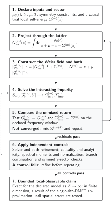
Single-site DMFT self-consistency and validation. Solid arrows are required update steps; dashed exits are checks, not extra approximations. Passing the loop and solver controls yields exact local observables only in the infinite-coordination limit, and yields observables of the single-site-DMFT approximation in finite dimension. The diagram is schematic and not to scale.

Open the loop at full size or download its semantic record. The ordered calculation is:

1. Choose the noninteracting density of states $\rho_0(\epsilon)=N^{-1}\sum_{\mathbf k}\delta(\epsilon-\epsilon_{\mathbf k})$, $U$, $\mu$, $T$, and the allowed symmetry sector, with $\int\mathrm d\epsilon\,\rho_0(\epsilon)=1$. Here $\epsilon_{\mathbf k}$ is the noninteracting band dispersion. Start from a causal trial $\Sigma^{(m)}(z)$; in a coexistence study, continue metallic and insulating seeds separately.

2. Reinsert that local self-energy into the lattice:

   $$\begin{aligned} G_{\mathrm{loc}}^{(m)}(z) &=\frac1N\sum_{\mathbf k} \frac1{z+\mu-\epsilon_{\mathbf k}-\Sigma^{(m)}(z)}\\ &=\int\mathrm d\epsilon\, \frac{\rho_0(\epsilon)}{z+\mu-\epsilon-\Sigma^{(m)}(z)}. \end{aligned}$$

3. Construct the new Weiss field and hybridization:

   $$[\mathcal G_0^{(m)}]^{-1} =[G_{\mathrm{loc}}^{(m)}]^{-1}+\Sigma^{(m)}, \qquad \Delta^{(m)}=z+\mu-[\mathcal G_0^{(m)}]^{-1}.$$

4. Solve the interacting impurity defined by $\mathcal G_0^{(m)}$ to obtain $G_{\mathrm{imp}}^{(m)}$ and the unmixed returned self-energy

   $$\Sigma_{\mathrm{imp}}^{(m)} =[\mathcal G_0^{(m)}]^{-1}-[G_{\mathrm{imp}}^{(m)}]^{-1}.$$

5. If the fixed-point and physicality checks fail, update—for example,

   $$\Sigma^{(m+1)} =(1-\alpha)\Sigma^{(m)}+\alpha\Sigma_{\mathrm{imp}}^{(m)}, \qquad 0<\alpha\le1,$$

   and repeat. Mixing can stabilize an iteration, but it does not change the stationary DMFT equation.

Broken-symmetry calculations use the same logic but restore the appropriate spin, orbital, and sublattice matrix indices in the lattice Dyson equation and Weiss field Georges et al. 1996, §§ V.A–B, printed pp. 31–32, eqs. (88)–(97).

Residuals and errors that must stay separate

A reproducible calculation declares the Matsubara window $\mathcal W$, mixing rule, tolerance, and normalization. Define the symmetric normalized distance

$$d[X,Y;X_{\mathrm{floor}}] =\frac{\lvert X-Y\rvert} {\lvert X\rvert+\lvert Y\rvert+X_{\mathrm{floor}}}.$$

Two useful residuals are

$$R_G=\max_{n\in\mathcal W} d[G_{\mathrm{imp}}^{(m)},G_{\mathrm{loc}}^{(m)};G_{\mathrm{floor}}],$$ $$R_\Sigma=\max_{n\in\mathcal W} d[\Sigma_{\mathrm{imp}}^{(m)},\Sigma^{(m)};\Sigma_{\mathrm{floor}}],$$

with every function evaluated at $i\omega_n$. Here $G_{\mathrm{floor}}$ has inverse-energy units and $\Sigma_{\mathrm{floor}}$ has energy units. Comparing the unmixed returned self-energy with the input prevents a small mixing parameter from manufacturing an artificially small $R_\Sigma$.

Error layer	What is tested	What a pass does not establish
DMFT fixed point	$R_G$, $R_\Sigma$, frequency-window stability, branch continuation, and mixing independence	Accuracy of the impurity solve or physical stability of the branch
Impurity solve	Statistical error and autocorrelation, bath representation when discretized, time or energy resolution, Hilbert-space truncation, and an exact-limit or independent-solver benchmark	Convergence of the lattice feedback loop
Real-frequency inference	Covariance-aware continuation, prior or regularization variation, resolution tests, sum rules, and high-frequency moments	A unique spectrum merely because one continuation looks smooth

Continuous-time Monte Carlo removes a time-discretization error but retains statistical, autocorrelation, sign, estimator, and representation issues Gull et al. 2011, § II.2 and §§ IX–X. No solver family is certified by a small DMFT residual. The dedicated NRG and CT-QMC validity page develops the cross-solver error analysis. The chapter reduction map locates DMFT among independent solver routes, and the chapter validity table places these controls between the mapping and any physical claim.

Bethe-lattice checkpoint and its two branches

For the normalized semicircular noninteracting density of states,

$$\rho_0(\epsilon) =\frac{\sqrt{4t^{*2}-\epsilon^2}}{2\pi t^{*2}}, \qquad \lvert\epsilon\rvert\le2t^*, \qquad \int\mathrm d\epsilon\,\rho_0(\epsilon)=1,$$

the Hilbert transform collapses to

$$\Delta(z)=t^{*2}G_{\mathrm{loc}}(z), \qquad \mathcal G_0^{-1}(z)=z+\mu-\Delta(z).$$

This is the algebraic Bethe-DMFT self-consistency relation. For an arbitrary impurity self-energy, define $\xi(z)=z+\mu-\Sigma(z)$. Then

$$G_{\mathrm{loc}}(z) =\frac{1}{\xi(z)-t^{*2}G_{\mathrm{loc}}(z)},$$

so the physical lattice update is

$$G_{\mathrm{loc}}(z) =\frac{\xi(z)-\sqrt{\xi(z)^2-4t^{*2}}}{2t^{*2}}.$$

The square root is the analytic branch satisfying $\sqrt{\xi^2-4t^{*2}}\sim\xi$ and $G_{\mathrm{loc}}\sim1/\xi$ at large $\lvert\xi\rvert$; for $\operatorname{Im}z>0$, it also gives $\operatorname{Im}G_{\mathrm{loc}}(z)<0$. The equation is algebraic in the lattice step, but the interacting $\Sigma[\mathcal G_0,U]$ still comes from the impurity problem.

At $U=0$, $\Sigma=0$ and $\xi=\zeta\equiv z+\mu$, giving

$$t^{*2}G(z)^2-\zeta G(z)+1=0.$$

At the particle–hole-symmetric point, the unshifted Hubbard convention has $\mu=U/2$, so $U=0$ implies $\mu=0$. The physical root reproduces the semicircular density of states, its unit normalization, and the first large-frequency moment Georges et al. 1996, § II.C, printed pp. 20–21, eqs. (21)–(23), and Appendix A, printed p. 117, eqs. (A44)–(A46).

At half filling and zero temperature, converged paramagnetic branches can be distinguished by their low-frequency structure:

• A Fermi-liquid metal has $Z>0$ and, in the unshifted convention,

  $$\Sigma(i\omega)=\frac U2+(1-Z^{-1})i\omega+O(\omega^2).$$

• A Mott-insulating branch has a spectral gap and a self-energy pole,

  $$\Sigma(i\omega)-\frac U2\sim\frac{C}{i\omega}, \qquad C>0,$$

  so $G(i\omega)\to0$ as $\omega\to0$.

At nonzero temperature these are metal-like and insulator-like solutions identified by continuity and low-frequency observables, not two sharply distinct phases everywhere. In the coexistence region, controlled continuation from both converged branches is necessary. A spinodal is where the corresponding stationary DMFT solution ceases to exist—not merely where one chosen iteration stops converging.

From a fixed point to observables

Once the fixed point and solver checks pass, the impurity directly supplies local observables such as the density $n_\sigma=G_\sigma(0^-)=-G_\sigma(\beta^-)$ and double occupancy $\langle n_\uparrow n_\downarrow\rangle$. The minus sign follows from fermionic antiperiodicity. With the chapter convention,

$$A_{\mathrm{loc}}(\omega)=-2\operatorname{Im}G_{\mathrm{loc}}^R(\omega), \qquad \rho_{\mathrm{loc}}(\omega)=\frac{A_{\mathrm{loc}}(\omega)}{2\pi}.$$

Momentum-resolved one-particle quantities require the reconstructed lattice propagator $G(\mathbf k,z)=[z+\mu-\epsilon_{\mathbf k}-\Sigma(z)]^{-1}$. Two-particle response functions generally require impurity vertex information and the lattice Bethe–Salpeter reconstruction; an impurity susceptibility is not automatically the lattice uniform susceptibility.

On the real-frequency axis, scalar retarded functions must obey

$$-\operatorname{Im}\Delta^R(\omega)\ge0, \qquad -\operatorname{Im}\Sigma^R(\omega)\ge0.$$

For matrix-valued spin, orbital, or sublattice problems, the corresponding anti-Hermitian parts must be positive semidefinite:

$$-\frac{\Delta^R-\Delta^{R\dagger}}{2i}\succeq0, \qquad -\frac{\Sigma^R-\Sigma^{R\dagger}}{2i}\succeq0.$$

These sign tests are necessary, not sufficient: analyticity, Kramers–Kronig consistency, high-frequency moments, the spectral sum rule, and agreement between impurity and lattice density remain independent checks.

Coexistence and the evidence ceiling

In the symmetry-restricted, half-filled, single-band problem, paramagnetic DMFT at finite temperatures below its critical endpoint can have metal-like and insulator-like stationary solutions between $U_{c1}(T)$ and $U_{c2}(T)$. Their free energies cross at a first-order line $U_c(T)$ inside that coexistence region Georges et al. 1996, § VII.D.1, printed pp. 65–66, Fig. 33, and § VII.D.2, printed p. 67, eqs. (238)–(239). Following both seeds is a search strategy; locating a spinodal requires solver-, bath-, tolerance-, and mixing-stable continuation, while locating $U_c(T)$ requires thermodynamic-potential comparison. The first-order line terminates at $T=0$ at $U_{c2}(0)$, where the transition is continuous in this restricted problem Georges et al. 1996, § VII.E, printed pp. 70–71, eqs. (240)–(244).

On a half-filled bipartite lattice, antiferromagnetic order can preempt the paramagnetic transition Georges et al. 1996, § VII.D.3, printed p. 69 and Fig. 42. More generally, the allowed symmetry sector is part of the scientific claim, not a technical afterthought.

In the controlled infinite-coordination limit, a solver-controlled DMFT fixed point yields exact local observables of the stated model and symmetry sector. On a finite-dimensional lattice, it establishes properties only of the single-site-DMFT approximation. It does not become controlled in two dimensions merely because $U$ is large. When short-range spatial correlations or momentum differentiation matter, proceed to the cluster extensions.

Common pitfalls

Confusing the cavity propagator with the Weiss propagator. $G_{ij}^{(0)}$ belongs to an interacting lattice with site $0$ removed. $\mathcal G_0$ is the Gaussian bath propagator of the auxiliary impurity. The cavity construction determines the latter from the former only after the large-coordination reduction.

Calling iteration failure a spinodal. A fixed-point algorithm can fail because of mixing, solver noise, bath resolution, or conditioning while a stationary solution still exists. A physical spinodal must be stable against those numerical choices.

Treating locality as a strong-coupling statement. The controlled locality is an infinite-coordination result with scaled hopping. Large $U$ alone neither suppresses finite-dimensional spatial correlations nor licenses a local self-energy.

Exercises

Weiss-field update. Derive the Weiss-field update from the impurity Dyson equation and the DMFT fixed-point conditions.

Solution

The impurity Dyson equation is $G_{\mathrm{imp}}^{-1}=\mathcal G_0^{-1}-\Sigma_{\mathrm{imp}}$. At the DMFT fixed point, $G_{\mathrm{imp}}=G_{\mathrm{loc}}$ and $\Sigma_{\mathrm{imp}}=\Sigma$. Substitution gives $G_{\mathrm{loc}}^{-1}=\mathcal G_0^{-1}-\Sigma$, hence $\mathcal G_0^{-1}=G_{\mathrm{loc}}^{-1}+\Sigma$. This is a consequence of matching the impurity and lattice local problems, not an independent ansatz.

Physical Bethe branch. Derive the interacting Bethe-lattice update and select its physical root.

Solution

Insert $\Delta=t^{*2}G_{\mathrm{loc}}$ into $G_{\mathrm{loc}}^{-1}=z+\mu-\Sigma-\Delta$ and set $\xi=z+\mu-\Sigma$. Then $t^{*2}G_{\mathrm{loc}}^2-\xi G_{\mathrm{loc}}+1=0$. The root with the minus sign and the analytic square-root branch $\sqrt{\xi^2-4t^{*2}}\sim\xi$ gives $G_{\mathrm{loc}}\sim1/\xi$ and the correct retarded sign. The other root grows as $\xi/t^{*2}$ and violates spectral normalization.

Atomic limit. Take $t^*\to0$ in the Bethe self-consistency. What happens to the bath, and what remains nontrivial?

Solution

Because $\Delta=t^{*2}G_{\mathrm{loc}}$, the hybridization vanishes. The impurity becomes an isolated interacting Hubbard atom. Its local interaction, thermal occupations, and atomic poles remain nontrivial, but there is no dynamical exchange with a bath. This checks that DMFT contains both the noninteracting lattice and atomic limits.

Insulating branch. At half filling, use $\Sigma(i\omega)-U/2\sim C/(i\omega)$ to explain why $G(i\omega)\to0$.

Solution

For small $\omega$, the pole makes $\xi=i\omega+U/2-\Sigma\sim-C/(i\omega)$. The physical Bethe root behaves as $G\sim1/\xi$, hence $G(i\omega)\sim-i\omega/C\to0$. The vanishing local propagator is consistent with zero low-energy spectral weight, whereas a Fermi-liquid branch has finite quasiparticle weight.

Branch-versus-solver diagnosis. A calculation converges from a metallic seed but not from an insulating seed. May it claim that no insulating branch exists?

Solution

No. The failed run may reflect mixing, solver noise, bath resolution, a frequency-window choice, or a tolerance problem. One must first control those errors and document continuation of the stationary solution. Even after both spinodals are located, identifying the finite-temperature first-order line requires a thermodynamic-potential comparison; iteration stability is not a free-energy criterion.

Convergence is not causality. A run has tiny $R_G$ and $R_\Sigma$, but $-\operatorname{Im}\Delta^R(\omega)<0$ on part of the real axis and its spectral sum rule fails. Is the result acceptable?

Solution

No. The iteration has reached a numerical fixed point of its implemented map, but that fixed point is not a physical causal solution. The bath, solver, continuation, Dyson signs, and high-frequency treatment must be repaired before any observable is used.

Néel self-consistency. Restore the sublattice and spin labels for nearest-neighbor Bethe-lattice DMFT in a bipartite antiferromagnet.

Solution

Every neighbor of sublattice $A$ lies on $B$, so the cavity relation gives

$$\mathcal G_{0,A\sigma}^{-1}(z) =z+\mu-t^{*2}G_{B\sigma}(z), \qquad \mathcal G_{0,B\sigma}^{-1}(z) =z+\mu-t^{*2}G_{A\sigma}(z).$$

For a collinear Néel state without a uniform field, spin reversal followed by sublattice exchange gives $G_{A\sigma}=G_{B\bar\sigma}$, and likewise for $\Sigma$ and $\mathcal G_0$. Setting the two sublattices equal would impose the paramagnetic sector and erase the order one intended to test.

Finite-dimensional claim. A two-dimensional single-site-DMFT calculation passes every residual, causality, sum-rule, and impurity-solver test. State the strongest justified conclusion.

Solution

It establishes a solver-controlled local result of the single-site-DMFT approximation for the declared two-dimensional model and symmetry sector. It does not establish that the finite-dimensional lattice has a local self-energy or that the inferred phase survives spatial correlations. Those claims require cluster convergence or an independent finite-dimensional benchmark.

References

• Antoine Georges and Gabriel Kotliar, “Hubbard Model in Infinite Dimensions,” Physical Review B 45 (1992) 6479–6483, doi:10.1103/PhysRevB.45.6479.
• Antoine Georges, Gabriel Kotliar, Werner Krauth, and Marcelo J. Rozenberg, “Dynamical Mean-Field Theory of Strongly Correlated Fermion Systems and the Limit of Infinite Dimensions,” Reviews of Modern Physics 68 (1996) 13–125, doi:10.1103/RevModPhys.68.13.
• Emanuel Gull, Andrew J. Millis, Alexander I. Lichtenstein, Alexey N. Rubtsov, Matthias Troyer, and Philipp Werner, “Continuous-Time Monte Carlo Methods for Quantum Impurity Models,” Reviews of Modern Physics 83 (2011) 349–404, doi:10.1103/RevModPhys.83.349.
• Walter Metzner and Dieter Vollhardt, “Correlated Lattice Fermions in $d=\infty$ Dimensions,” Physical Review Letters 62 (1989) 324–327, doi:10.1103/PhysRevLett.62.324; erratum, Physical Review Letters 62 (1989) 1066, doi:10.1103/PhysRevLett.62.1066.