Optical Lattices and Hubbard-Model Realizations

An optical lattice programs a periodic potential, not an exact Hubbard Hamiltonian. The Hubbard parameters follow from a band projection with a specified Wannier convention and interaction calibration; higher bands, longer-range terms, confinement, loading dynamics, heating, and the imaging kernel determine the discrepancy between the programmed and realized models.

Required background. The fermionic Hubbard model and Mott regime supplies the target fermion Hamiltonian and its scales. The Bose–Hubbard superfluid–Mott transition supplies the bosonic target. What counts as a quantum simulation distinguishes programming, realization, and validation.

From an optical potential to Wannier parameters

For a separable standing-wave lattice,

$$V_{\mathrm{lat}}(\mathbf r) =\sum_{\alpha=1}^{d}V_\alpha\sin^2(k_\alpha x_\alpha), \qquad a_\alpha=\frac{\pi}{k_\alpha}, \qquad E_{R,\alpha}=\frac{\hbar^2k_\alpha^2}{2m}.$$

Let $w_i(\mathbf r)$ be a localized Wannier orbital of the selected band. Projecting the continuum Hamiltonian gives

$$H_{\mathrm{Hub}}= -\sum_{\langle ij\rangle,\sigma} \left(t_{ij}c_{i\sigma}^\dagger c_{j\sigma} +\mathrm{h.c.}\right) +U\sum_i n_{i\uparrow}n_{i\downarrow} +\sum_i(V_i-\mu)n_i,$$

with

$$t_{ij}=-\int\mathrm d^3r\,w_i^* \left[-\frac{\hbar^2\nabla^2}{2m}+V_{\mathrm{lat}}\right]w_j, \qquad U=g\int\mathrm d^3r\,\lvert w_i\rvert^4, \quad g=\frac{4\pi\hbar^2a_s}{m}.$$

The phase of each Wannier orbital can change the sign convention for $t_{ij}$, but gauge-invariant fluxes and the band dispersion cannot. For a deep isotropic simple-cubic lattice of depth $s=V_0/E_R$, harmonic-well asymptotics give

$$\frac{t}{E_R}\simeq \frac{4}{\sqrt\pi}s^{3/4}e^{-2\sqrt s}, \qquad \frac{U}{E_R}\simeq \sqrt{\frac8\pi}\,k_La_s\,s^{3/4}.$$

These formulas are useful estimates, not calibration substitutes. The optical-lattice reduction to a Bose–Hubbard model was formulated by Jaksch et al. 1998, main text, and the broader continuum-to-lattice hierarchy is reviewed by Bloch, Dalibard, and Zwerger 2008, §§V–VI. Band-structure and Wannier calculations using the measured beam geometry are required when $s$ is moderate, axes are unequal, the potential is nonseparable, or interaction-induced orbital deformation matters.

The structure figure shows where the projection sits. Inspect the correction branch: calibrating $t$ and $U$ is necessary, but the realized Hamiltonian also contains every retained term at the uncertainty level relevant to the claimed observable.

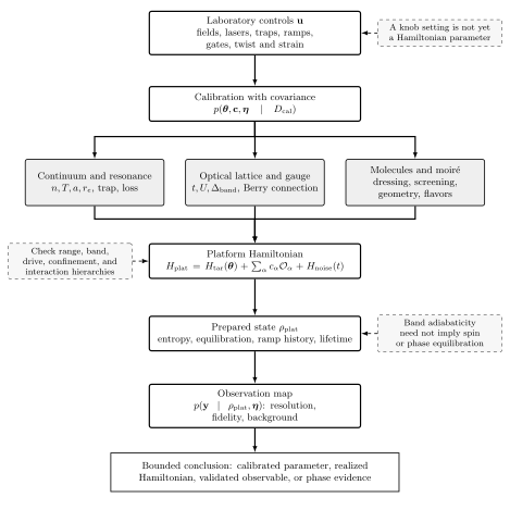
Optical-lattice realization in the platform-to-model chain. Potential calibration, band projection, state loading, and observable reconstruction are separate transformations with separate uncertainties. Original schematic, not to scale; experimental status is bounded through 10 August 2026.

The correction hierarchy

Let $\Delta_{\mathrm{band}}$ be the gap from the selected band to the nearest excluded band. A single-band reduction requires

$$\epsilon_{\mathrm{band}} =\frac{\max(t,U,k_BT,\hbar/t_{\mathrm{ramp}})} {\Delta_{\mathrm{band}}}\ll1$$

for the processes used. This condition must be checked locally in an inhomogeneous lattice and during the full ramp. A small final ratio does not undo nonadiabatic excitation generated while a gap was narrow.

The effective Hamiltonian generally also contains

$$\delta H= -\sum_{\langle\!\langle ij\rangle\!\rangle,\sigma} \left(t'_{ij}c_{i\sigma}^\dagger c_{j\sigma} +\mathrm{h.c.}\right) +\sum_{\langle ij\rangle}V_{ij}n_in_j +\sum_{\langle ij\rangle,\sigma} \left[ X_{ij}(n_{i\bar\sigma}+n_{j\bar\sigma}) c_{i\sigma}^\dagger c_{j\sigma} +\mathrm{h.c.} \right] +\cdots .$$

Next-neighbor tunneling $t'$, off-site interactions $V_{ij}$, density-assisted tunneling $X_{ij}$, multibody loss, and spatial variations in $t$ or $U$ should be bounded against the smallest effect being interpreted. Near strong coupling the spin scale $J_{\mathrm ex}=4t^2/U$ is much smaller than $t$, so a percent-level Hamiltonian correction can be large relative to $J_{\mathrm ex}$.

For a smooth trap, the site chemical potential is $\mu_i=\mu_0-V_{\mathrm{tr}}(\mathbf r_i)$ and LDA can reconstruct homogeneous observables from shells. Sharp walls, small ordered domains, and slow mass transport violate that step. Loading entropy is equally important: an isentropic ramp can heat or cool in units of $t$ because the density of states changes, and “adiabatic with respect to the band gap” does not imply equilibrium with respect to spin exchange. Esslinger 2010, §§2–5 reviews these Fermi–Hubbard preparation and measurement scales.

Observable maps and current benchmark evidence

A quantum gas microscope measures an image distribution. Light-assisted collisions may project doublons to even parity; hopping or loss during fluorescence changes occupations; spin removal has its own fidelity; finite numerical aperture mixes nearby sites. If $n_i$ is the premeasurement occupation and $y_j$ the recorded outcome, validation needs a response matrix

$$P(\mathbf y\mid\mathbf n,\boldsymbol\eta),$$

with nuisance parameters $\boldsymbol\eta$ calibrated on held-out states. Density, doublon fraction, spin correlations, string correlators, and snapshots require different inversions and covariances.

Xu et al. 2025, Methods and source data provide a current high-control example: measured lattice depths and magnetic fields were converted to $t$ and $U$, trap potentials were independently reconstructed, preparation ramps were specified, and correlation-based thermometry was compared with numerical calculations. At half filling, numerically controlled comparisons were stronger than at finite doping, where constrained-path calculations introduced a separate model uncertainty. The durable conclusion is therefore observable- and parameter-window specific, not a universal certification of the doped Hubbard phase diagram.

Evidence and platform capabilities on this page are current through 10 August 2026. Later calibrations, corrections, and phase inferences belong in the Quantum Matter and Emergence Research synthesis. The canonical cold-atom and synthetic-matter claim test matrix records the Hamiltonian term, scale hierarchy, preparation, readout, discrepancy, and evidence ceiling. A reproducible verification workflow propagates the calibration covariance into model observables.

Exercise

Estimate a Hubbard hierarchy. In a cubic lattice take $s=8$ and $k_La_s=0.05$. Use the deep-lattice formulas to estimate $t/E_R$, $U/E_R$, and $U/t$. Compare them with the harmonic band gap $\Delta_{\mathrm{band}}\simeq2\sqrt{s}\,E_R$.

Solution

Here $s^{3/4}\simeq4.76$ and $e^{-2\sqrt s}\simeq3.49\times10^{-3}$. Therefore

$$\frac{t}{E_R}\simeq \frac4{\sqrt\pi}(4.76)(3.49\times10^{-3}) \simeq0.0375,$$

and

$$\frac{U}{E_R}\simeq \sqrt{\frac8\pi}(0.05)(4.76) \simeq0.380, \qquad \frac Ut\simeq10.1.$$

The estimated band gap is $\Delta_{\mathrm{band}}/E_R\simeq5.66$, so $t/\Delta_{\mathrm{band}}\simeq0.0066$ and $U/\Delta_{\mathrm{band}}\simeq0.067$. The hierarchy is plausibly single-band, but the asymptotic formulas, confinement-renormalized interaction, ramp excitation, and smaller scale $J_{\mathrm ex}=4t^2/U\simeq0.0148E_R$ still require explicit checks.

References

• Bloch, I., Dalibard, J., and Zwerger, W. (2008). “Many-body physics with ultracold gases.” Reviews of Modern Physics 80, 885–964. doi:10.1103/RevModPhys.80.885.
• Esslinger, T. (2010). “Fermi–Hubbard physics with atoms in an optical lattice.” Annual Review of Condensed Matter Physics 1, 129–152. doi:10.1146/annurev-conmatphys-070909-104059.
• Jaksch, D., Bruder, C., Cirac, J. I., Gardiner, C. W., and Zoller, P. (1998). “Cold bosonic atoms in optical lattices.” Physical Review Letters 81, 3108–3111. doi:10.1103/PhysRevLett.81.3108.
• Xu, M., Kendrick, L. H., Kale, A., Gang, Y., Feng, C., Zhang, S., Young, A. W., Lebrat, M., and Greiner, M. (2025). “A neutral-atom Hubbard quantum simulator in the cryogenic regime.” Nature 642, 909–915. doi:10.1038/s41586-025-09112-w.