Gauge-Invariant Meissner Response and Superfluid Weight

The Meissner effect is an equilibrium statement: a weak, static transverse magnetic field is screened in the bulk. Microscopically, the screening coefficient is the part of the current response left after the paramagnetic current correlator and the diamagnetic contact term are combined in one gauge-consistent approximation. A pairing gap, an anomalous propagator, or even a zero-frequency conductivity delta function is not enough by itself. The decisive object is the static transverse kernel and the penetration depth extracted from it. We work in linear response about a vortex-free Meissner state; the explicit field profile below assumes a simply connected, local three-dimensional bulk, while thin films, anisotropy, and nonlocality are identified separately.

Required background. Gauge redundancy and observables, the gauge-invariant Higgs mechanism, and Kubo response supply the field, observable, and limit conventions.

Helpful background. The page on Nambu–Gor’kov propagators supplies the paired Green function and explains why the response vertex must be matched to the self-energy.

From minimal coupling to the transverse kernel

Begin with a clean, spin-degenerate band in thermal equilibrium. Write its dispersion as $\varepsilon_{\mathbf k}$ and $\xi_{\mathbf k}=\varepsilon_{\mathbf k}-\mu$, and let $q$ be the constituent fermion’s signed charge. Bold $\mathbf p$ below is the probe wavevector; it is not the charge. The final linear response depends on $q^2$, so an electron may be described by $q=-e$ without changing the formulas below. We use $\hbar=k_{\mathrm B}=1$, hence $\beta=1/T$, in the matter calculation, take $\mathbf k$ to be canonical momentum, and restore SI electromagnetic units when extracting a penetration depth. Repeated spatial indices are summed.

Expanding the minimally coupled one-body Hamiltonian to second order in a slowly varying vector potential gives the uniform vertices

$$H[\mathbf A] =H[0]-\mathcal J_i^{\mathrm p}A_i +\frac12\mathcal T_{ij}A_iA_j+O(A^3),$$

with

$$\begin{aligned} \mathcal J_i^{\mathrm p} &=q\sum_{\mathbf k,\sigma}v_{\mathbf k i} c^\dagger_{\mathbf k\sigma}c_{\mathbf k\sigma}, &v_{\mathbf k i}&=\frac{\partial\varepsilon_{\mathbf k}}{\partial k_i},\\ \mathcal T_{ij} &=q^2\sum_{\mathbf k,\sigma}m^{-1}_{\mathbf k,ij} c^\dagger_{\mathbf k\sigma}c_{\mathbf k\sigma}, &m^{-1}_{\mathbf k,ij}&= \frac{\partial^2\varepsilon_{\mathbf k}}{\partial k_i\partial k_j}. \end{aligned}$$

The calligraphic quantities are extensive total-current operators. If $V$ is the spatial volume, the measured current density and the intensive contact kernel are

$$j_i=\frac{\langle\mathcal J_i\rangle}{V}, \qquad D^{\mathrm{dia}}_{ij}=\frac{\langle\mathcal T_{ij}\rangle}{V}.$$

The first band derivative produces the paramagnetic current vertex; the second produces the diamagnetic contact term. For $\varepsilon_{\mathbf k}=\mathbf k^2/(2m)$, $D^{\mathrm{dia}}_{ij}=nq^2\delta_{ij}/m$. On a lattice it is instead a Brillouin-zone average of the band curvature and must not be replaced by $nq^2/m$.

At finite probe momentum, $\mathcal J_i^{\mathrm p}(\mathbf p)$ denotes the exact vertex obtained by differentiating the fully gauge-coupled Hamiltonian; it reduces to the displayed operator as $\mathbf p\to0$. Using that exact finite-$\mathbf p$ vertex, rather than guessing a shifted continuum velocity on a lattice, is part of satisfying the Ward identity.

There is one important units translation. If a solid-state band is tabulated against a wavevector $\mathbf k$ in inverse metres rather than a canonical momentum, then minimal coupling is $\mathbf k\mapsto\mathbf k-q\mathbf A/\hbar$ and

$$v_{\mathbf k i}^{\mathrm{phys}} =\frac{1}{\hbar}\frac{\partial\varepsilon_{\mathbf k}}{\partial k_i}, \qquad (m^{-1}_{\mathbf k})_{ij}^{\mathrm{phys}} =\frac{1}{\hbar^2} \frac{\partial^2\varepsilon_{\mathbf k}}{\partial k_i\partial k_j}.$$

Dropping these factors is a units error, not a convention change. The measure must be translated with the same care: a wavevector integral uses $\mathrm d^{d_s}k/(2\pi)^{d_s}$, whereas an integral over canonical momentum $\mathbf p_c=\hbar\mathbf k$ uses $\mathrm d^{d_s}p_c/(2\pi\hbar)^{d_s}$.

Define the Euclidean paramagnetic susceptibility and total kernel by

$$\begin{aligned} \chi^{\mathrm p}_{ij}(Q) &=\frac{1}{V}\int_0^\beta\!\mathrm d\tau\, e^{i\Omega_m\tau} \left\langle \mathcal T_\tau \mathcal J_i^{\mathrm p}(\tau,\mathbf p) \mathcal J_j^{\mathrm p}(0,-\mathbf p)\right\rangle_{\!c},\\ K_{ij}(Q)&=D^{\mathrm{dia}}_{ij}-\chi^{\mathrm p}_{ij}(Q), \qquad j_i(Q)=-K_{ij}(Q)A_j(Q). \end{aligned}$$

Here $Q=(i\Omega_m,\mathbf p)$ and $\mathcal T_\tau$ orders operators in imaginary time. Thus every term in $K$ has the units of an intensive current-density response.

Equivalently, a common retarded convention writes $K^R=D^{\mathrm{dia}}+\Pi^R$, where the static paramagnetic contribution $\Pi^R$ is negative. Stating this sign convention matters: changing the definition of $\Pi$ without changing the plus sign would turn screening into an apparent instability.

For an isotropic medium at nonzero $\mathbf p$, decompose

$$K_{ij}=K_T\left(\delta_{ij}-\frac{p_ip_j}{\mathbf p^2}\right) +K_L\frac{p_ip_j}{\mathbf p^2}.$$

In an anisotropic medium, retain the transverse projector $P^T_{ij}=\delta_{ij}-\hat p_i\hat p_j$ on both sides of the full tensor instead of forcing it into two scalars. The equilibrium transverse weight is

$$\big[D_s^{(T)}(\hat{\mathbf p})\big]_{ij} =\lim_{p\to0} P^T_{ia}K_{ab}(p\hat{\mathbf p},i\Omega_m=0)P^T_{bj}.$$

This test requires at least two spatial dimensions. First take the thermodynamic limit at fixed sample shape and fixed nonzero $\mathbf p$; then set the frequency to zero, project transverse to $\mathbf p$, and finally take $p\to0$. In a homogeneous local medium, write the intrinsic helicity-modulus tensor as $D_{s,ij}$. The electromagnetic response for propagation direction $\hat{\mathbf p}$ is its projected tensor $P^T D_sP^T$ and therefore remains direction-dependent in an anisotropic material; only in an isotropic medium does it reduce to $D_s\delta_{ij}$ on every transverse subspace. The opposite, spatially uniform dynamic limit measures ideal transport and can remain nonzero in a nonsuperconducting system with protected ballistic current. Scalapino, White, and Zhang 1993, §II, pp. 7996–7998, Eqs. (8), (11)–(12), and (20)–(21) formulates this distinction as a practical criterion for metals, insulators, and superconductors.

Gauge consistency is stronger than transversality of one selected component. The full density-current response must obey $Q_\mu K^{\mu\nu}=0$ and the associated sum rules. At a self-consistent BCS saddle, the contact term and paired bubble reconstruct the transverse result below. Longitudinal response also requires the phase collective vertex. Anderson 1958, pp. 827–835 shows how that coherent phase sector reconciles BCS response with gauge invariance and is shifted to the plasma scale by long-range Coulomb forces. More generally, a dressed propagator with a bare vertex is not a conserving approximation: the vertex must be generated from the same interaction or self-energy functional. Nambu 1960, abstract states the generalized Ward relation between vertex parts and self-energy in the paired state, while Baym and Kadanoff 1961, abstract connects matched vertices to conservation laws and sum rules.

The clean BCS kernel

Now specialize to an isolated spin-degenerate band with $\xi_{\mathbf k}=\xi_{-\mathbf k}$, homogeneous zero-momentum singlet pairing, and a self-consistent momentum-independent gap $\Delta$. In the local static transverse limit, the quasiparticle energy is

$$E_{\mathbf k}=\sqrt{\xi_{\mathbf k}^2+|\Delta|^2}, \qquad f(E)=\frac{1}{e^{\beta E}+1}.$$

We write $f'(E)=\mathrm df/\mathrm dE$. These assumptions are what make the following compact single-band formula possible; it is not the generic multiband or momentum-dependent-gap kernel.

The total occupation of the two spin states at momentum $\mathbf k$ is

$$n_{\mathbf k} =1-\frac{\xi_{\mathbf k}}{E_{\mathbf k}} \tanh\!\left(\frac{E_{\mathbf k}}{2T}\right).$$

The short microscopic step is worth displaying. In the Nambu basis used on the prerequisite page,

$$\mathcal G^{-1}(\mathbf k,i\omega_n) =i\omega_n\tau_0-\xi_{\mathbf k}\tau_3 -\operatorname{Re}\Delta\,\tau_1 +\operatorname{Im}\Delta\,\tau_2,$$

and the local paramagnetic current vertex is $\Gamma_i=qv_{\mathbf k i}\tau_0$. The fermion-loop sign and the trace over the two Nambu branches give

$$\begin{aligned} \chi^{\mathrm p}_{ij} &=-q^2T\sum_n\int_{\mathbf k}v_{\mathbf k i}v_{\mathbf k j} \operatorname{tr}\!\left[\mathcal G(\mathbf k,i\omega_n)^2\right]\\ &=-q^2\int_{\mathbf k}v_{\mathbf k i}v_{\mathbf k j} \big[f'(E_{\mathbf k})+f'(-E_{\mathbf k})\big]\\ &=-2q^2\int_{\mathbf k}v_{\mathbf k i}v_{\mathbf k j}f'(E_{\mathbf k}). \end{aligned}$$

The last factor of two is already the contribution of the $\pm E_{\mathbf k}$ branches in this reduced spin-Nambu block; adding a second spin factor would double count it. In the local transverse limit, the contact term and this thermally excited-quasiparticle bubble give

$$\begin{aligned} D^{\mathrm{dia}}_{ij} &=q^2\int_{\mathbf k}m^{-1}_{\mathbf k,ij}\,n_{\mathbf k},\\ \chi^{\mathrm p}_{ij} &=-2q^2\int_{\mathbf k}v_{\mathbf k i}v_{\mathbf k j} \,f'(E_{\mathbf k}), \end{aligned} \qquad \int_{\mathbf k}\equiv\int\frac{\mathrm d^{d_s} k}{(2\pi)^{d_s}},$$

where $d_s$ is the number of spatial dimensions. Because $f'(E)<0$, $\chi^{\mathrm p}$ is positive and subtracts from the diamagnetic response. The clean BCS result is therefore

$$\boxed{ D_{s,ij}(T) =q^2\int_{\mathbf k} \left[ m^{-1}_{\mathbf k,ij} \left(1-\frac{\xi_{\mathbf k}}{E_{\mathbf k}} \tanh\frac{E_{\mathbf k}}{2T}\right) +2v_{\mathbf k i}v_{\mathbf k j}f'(E_{\mathbf k}) \right]. }$$

This equation displays the cancellation that a calculation must pass. In the normal state, integration by parts turns the band-curvature term into the equal paramagnetic term, so $\lim_{p\to0}K_T(\mathbf p,0)=0$. This does not forbid an $O(p^2)$ orbital-susceptibility term at finite momentum. In a fully gapped state at $T=0$, $f'(E_{\mathbf k})=0$: no quasiparticles remain to cancel the contact term. For a homogeneous, one-component, parabolic Galilean-invariant continuum,

$$D_{s,ij}(0)=\frac{nq^2}{m}\delta_{ij}.$$

For a periodic Brillouin zone, or a continuum whose boundary term vanishes, one more integration by parts rewrites the same uniform-gap answer as

$$D_{s,ij} =q^2\int_{\mathbf k}v_{\mathbf k i}v_{\mathbf k j} \frac{|\Delta|^2}{E_{\mathbf k}^2} \left[ \frac{1}{E_{\mathbf k}}\tanh\frac{E_{\mathbf k}}{2T} +2f'(E_{\mathbf k}) \right].$$

At fixed $T>0$, the square bracket has the small-$E$ expansion

$$\frac{1}{E}\tanh\frac{E}{2T}+2f'(E) =\frac{E^2}{12T^3}+O\!\left(\frac{E^4}{T^5}\right),$$

so the kernel vanishes as $O(|\Delta|^2)$ under the regularity assumptions above. The order of limits matters. At $T=0$,

$$\lim_{|\Delta|\to0^+} \frac{|\Delta|^2}{(\xi^2+|\Delta|^2)^{3/2}} =2\delta(\xi),$$

and a Galilean continuum retains $\lim_{|\Delta|\to0^+}D_s=nq^2/m$, whereas the exact normal state has $D_s(\Delta=0)=0$. This is the nonanalytic gapless-Fermi-surface endpoint associated with the Cooper instability, not a contradiction. The kernel also shows why low-temperature penetration-depth measurements are sensitive to the gap minimum: a full gap produces an exponentially small quasiparticle depletion, whereas symmetry-enforced nodes give power laws whose exponent depends on dimension, node geometry, disorder, and current matrix elements; Hirschfeld and Goldenfeld 1993, abstract exhibits the linear-to-quadratic crossover caused by strong impurity scattering in a two-dimensional $d$-wave state. The original BCS calculation keeps both current pieces and also derives the nonlocal Pippard kernel; see Bardeen, Cooper, and Schrieffer 1957, §V, pp. 1192–1198.

The simple formula is not universal. A lattice lacks the Galilean identity $D_s(0)=nq^2/m$. In multiband systems, interband current matrix elements generate a geometric contribution that can survive even when a band is flat; Liang et al. 2017, §§II–III separates this term from the conventional intraband contribution. Momentum-dependent gaps require the matching vertex, and disorder changes both propagators and vertices. Anderson protection of a gap or transition temperature does not license dropping impurity ladders from the response; Mattis and Bardeen 1958, pp. 412–417 develops the corresponding nonlocal electrodynamics. The invariant procedure is to differentiate the gauge-coupled Hamiltonian and evaluate the resulting contact and correlation terms consistently.

From superfluid weight to magnetic screening

At wavelengths long compared with the nonlocality scale, the bulk transverse response is local:

$$\mathbf j_T=-D_s\mathbf A_T.$$

This coefficient is the charged version of the pair-phase helicity modulus. If $\Upsilon_{ij}$ is defined by the pair-phase twist and each constituent has charge $q$, then the pair has charge $2q$ and

$$F_\theta =\frac12\int\mathrm d^{d_s} x\, \Upsilon_{ij} \left(\partial_i\theta-\frac{2q}{\hbar}A_i\right) \left(\partial_j\theta-\frac{2q}{\hbar}A_j\right), \qquad D_{s,ij}=\frac{4q^2}{\hbar^2}\Upsilon_{ij}.$$

In a Galilean continuum, $\Upsilon=\hbar^2n_s/(4m)$ when $n_s$ counts constituent particles, so the translation gives $D_s=n_sq^2/m$. For a homogeneous, one-component, Galilean-invariant superfluid ground state, $n_s=n$ at $T=0$, reproducing the microscopic BCS result. Writing $D_s=\Upsilon$ without declaring a pair-normalized source would miss this charge-two factor.

Now restore $D_s$ as a physical three-dimensional electrical-current-density kernel in SI units. In transverse gauge, $\boldsymbol\nabla\cdot\mathbf A=0$, use $\mathbf B=\boldsymbol\nabla\times\mathbf A$, static Ampère’s law $\boldsymbol\nabla\times\mathbf B=\mu_0\mathbf j$, and $\mathbf j=-D_s\mathbf A$. Then

$$-\boldsymbol\nabla^2\mathbf A =-\mu_0D_s\mathbf A,$$

and taking a curl gives

$$\boldsymbol\nabla^2\mathbf B=\lambda_L^{-2}\mathbf B, \qquad \lambda_L^{-2}=\mu_0D_s.$$

For a planar half-space $x>0$ with $\mathbf B=B_z(x)\hat{\mathbf z}$ parallel to its surface, the bounded solution and screening current are

$$B_z(x)=B_0e^{-x/\lambda_L}, \qquad j_y(x)=-\frac{1}{\mu_0}\frac{\mathrm dB_z}{\mathrm dx} =\frac{B_0}{\mu_0\lambda_L}e^{-x/\lambda_L}.$$

A positive $D_s$ therefore establishes equilibrium magnetic screening. The current is concentrated within a few penetration depths and integrates to $\int_0^\infty j_y\,\mathrm dx=B_0/\mu_0$, exactly the sheet current required by the magnetic-field jump.

For an anisotropic crystal, screening lengths are eigenmodes of the transverse Maxwell-response operator for the chosen surface orientation; one cannot generally interpret every component of $\mu_0D_{s,ij}$ as an independent componentwise penetration depth. Dimensionality matters too. A film of thickness $t\ll\lambda_L$ has sheet weight $D_s^{(2D)}=tD_s^{(3D)}$ and, in a symmetric vacuum environment, Pearl scale

$$\Lambda_P=\frac{2}{\mu_0D_s^{(2D)}} =\frac{2\lambda_L^2}{t},$$

rather than the three-dimensional bulk exponential; see Pearl 1964, pp. 65–66. A one-dimensional wire has no intrinsic bulk transverse Meissner limit, so its magnetic response must be solved together with the embedding geometry.

The local London equation is itself a limit. In a clean superconductor with coherence length $\xi_0$ comparable to or larger than $\lambda_L$, or whenever the field varies on scales $|\mathbf p|\xi_0\gtrsim1$, one must retain $K_T(\mathbf p,0)$ rather than replace it by $D_s$. Surface scattering and sample geometry then enter the Pippard screening problem. BCS separates the nonlocal kernel, London limit, and plane-surface problem in Bardeen, Cooper, and Schrieffer 1957, Eqs. (5.37), (5.42), (5.46), and (5.51)–(5.53), pp. 1194–1195.

Why optical delta weight is a different limit

Optics probes a different continuation. With the retarded convention above,

$$\sigma_{ij}(\omega) =\frac{i}{\omega+i0}\,K^R_{ij}(\mathbf 0,\omega),$$

For a chosen unit polarization $\hat{\mathbf e}$, define the uniform current kernel $K^R_{ee}=e_iK^R_{ij}e_j$ and the corresponding optical weight $D_{\mathrm{opt}}^{(e)}$; below the polarization label is suppressed when no ambiguity can arise. This avoids calling a component “transverse” at exactly $\mathbf p=0$, where no momentum direction exists.

An ideal zero-frequency weight then appears as

$$\operatorname{Re}\sigma(\omega) =\pi D_{\mathrm{opt}}\delta(\omega) +\sigma_{\mathrm{reg}}(\omega).$$

$D_{\mathrm{opt}}$ is a dynamic-limit weight, not the definition of $D_s$. A nonsuperconducting state can have a Drude delta function when its current overlaps an exactly conserved quantity and no effective relaxation channel removes that overlap—for example, in a Galilean-invariant continuum or a collisionless mean-field model—while its equilibrium Meissner weight remains zero. Cleanliness alone is not enough on an interacting lattice because Umklapp can relax current. Under the same no-relaxation qualification, finite-temperature superconducting quasiparticles can contribute to the optical delta weight in addition to the condensate response.

The figure makes the two response paths and their physical consequences visible. In the upper panel, inspect how the field and its supporting current share one penetration-depth scale. In the lower panel, follow each arrow to the origin and note which variable was set to zero first.

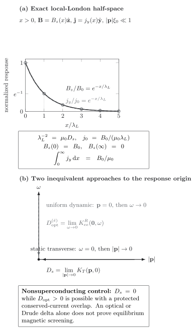
A positive local static transverse kernel gives the exact half-space profiles $B_z/B_0=j_y/j_0=e^{-x/\lambda_L}$, with $j_0=B_0/(\mu_0\lambda_L)$. The solid static-transverse path to the response origin defines $D_s$ and magnetic screening; the dashed uniform-dynamic path defines $D_{\mathrm{opt}}$ and can remain finite without superconductivity when current has a protected conserved overlap. Panel (a) is exact under the stated isotropic bulk London assumptions; panel (b) is schematic and not to scale.

Download the figure data (CSV) or its complete semantic record (JSON).

To state the optical sum rule without hiding ballistic weight, write $D_{\delta,n}$ and $D_{\delta,s}$ for the complete normal- and superconducting-state delta coefficients. When the two spectra have the same total intraband optical sum—equivalently, the same relevant diamagnetic or stress-tensor expectation in one normalization—

$$\frac{2}{\pi}\int_{0^+}^{\infty}\!\mathrm d\omega\, \left[ \sigma_{1,n}^{\mathrm{reg}}(\omega) -\sigma_{1,s}^{\mathrm{reg}}(\omega) \right] =D_{\delta,s}-D_{\delta,n}.$$

When this separation is well defined, define the residual superconducting ballistic contribution operationally by $D_{\mathrm{qp},s}\equiv D_{\delta,s}-D_s$, and write the normal ballistic weight as $D_{\delta,n}=D_n$. Then

$$D_s =\frac{2}{\pi}\int_{0^+}^{\infty}\!\mathrm d\omega\, \left[ \sigma_{1,n}^{\mathrm{reg}}-\sigma_{1,s}^{\mathrm{reg}} \right] +D_n-D_{\mathrm{qp},s}.$$

The familiar Ferrell–Glover–Tinkham missing-area formula follows when momentum relaxation removes both extra delta weights, or when $D_n=D_{\mathrm{qp},s}$ so that they cancel. Equal carrier density and the same bare band Hamiltonian guarantee the equal-sum premise in a parabolic Galilean continuum, but not on a lattice: the diamagnetic stress expectation can change between the normal and superconducting states. In general the right-hand side of the regular missing-area equation is $D_{\delta,s}-D_{\delta,n}+D^{\mathrm{dia}}_n-D^{\mathrm{dia}}_s$; the displayed equation is its equal-sum specialization. In a Galilean system without relaxation at $T=0$, instead, $D_n=D_s=nq^2/m$ and both regular parts can vanish: the regular missing area is zero even though the Meissner weight is finite. The factor $2/\pi$ follows from integrating a full-line term $\pi D_\delta\delta(\omega)$ over positive frequencies. A finite experimental cutoff, interband transfer, temperature-dependent lattice stress expectation, or an unresolved narrow Drude peak can spoil the naive missing-area estimate without invalidating gauge invariance. The original sum-rule observation is Ferrell and Glover 1958, pp. 1398–1399; its use to determine screening depth is developed in Tinkham and Ferrell 1959, pp. 331–333.

The names are close enough to invite confusion, so keep their definitions beside their claims:

Quantity	Definition or limit	What it establishes	Possible in an ordinary charged normal metal?
$D_s$	$\lim_{p\to0}K_T(\mathbf p,0)$ after the thermodynamic and transverse steps	Equilibrium transverse rigidity	No
$D_{\mathrm{Drude}}$	Spatially uniform dynamic limit with a protected current overlap	Ideal transport without relaxation	Yes, conditionally
$\Upsilon$	Curvature of free energy under a pair-phase twist	Phase rigidity before charge normalization	No
$\lambda_L^{-2}$	$\mu_0D_s$ for a local three-dimensional bulk	Exponential magnetic attenuation	No
$D_\delta$	Complete coefficient of $\pi\delta(\omega)$ in $\operatorname{Re}\sigma$	Zero-frequency spectral weight	Yes, conditionally

What a valid calculation must keep fixed

Check	Required calculation	Failure if omitted
Contact term	Differentiate the gauge-coupled dispersion twice.	A normal metal falsely acquires a Meissner kernel.
Conserving vertex	Generate the response vertex consistently with the self-energy and gap equation.	The Ward identity or longitudinal sum rule fails.
Order of limits	Take the thermodynamic limit, evaluate $\omega=0$, project transverse to $\mathbf p$, then take $\mathbf p\to0$.	A ballistic Drude weight is mislabeled as magnetic screening.
Band structure	Use $\partial_{k_i}\partial_{k_j}\varepsilon_{\mathbf k}$ and the actual current matrix elements.	The continuum value $nq^2/m$ is incorrectly imposed on a lattice.
Momentum units	Distinguish canonical momentum from wavevector and restore the required $\hbar^{-1}$ factors.	The current vertex, mass tensor, and penetration depth carry the wrong units.
Disorder	Dress both Green functions and impurity vertices in the same scheme.	The dirty-limit penetration depth and spectral weight are inconsistent.
Geometry and nonlocality	Compare $\xi_0$, mean free path, $\lambda_L$, thickness, and probe wavevector.	A Pippard or thin-film field profile is fitted by a local bulk exponential.
Optical sum	Include the complete relevant frequency range and residual zero-frequency weight.	Missing spectral area is over- or under-assigned to the condensate.

The structure map places this response gate between the Nambu calculation and the magnetic observable.

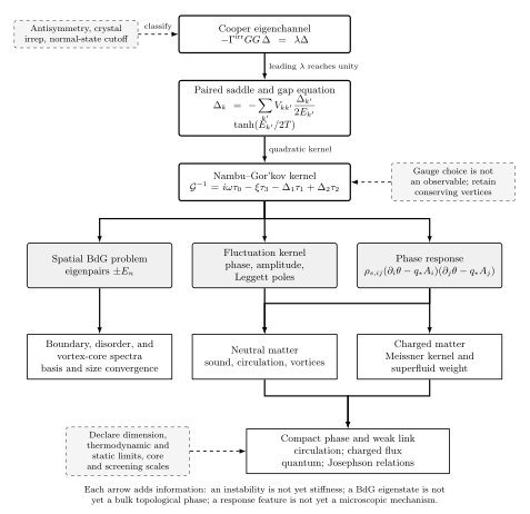
The paired saddle feeds a Nambu response calculation, which must pass the conserving-vertex and phase-stiffness gates before the chapter reaches gauge-invariant Meissner screening. Original chapter-orientation schematic, not to scale.

See the paired-matter claim test matrix for the independent checks that separate a paired saddle, phase rigidity, and magnetic screening. The structure-map JSON and claim-matrix JSON expose the same relations in structured form.

Common pitfalls

A gap is not a Meissner test. A pairing gap or anomalous propagator establishes a paired one-particle structure, not equilibrium transverse rigidity. The contact term, correlation kernel, vertex consistency, and static transverse limit still have to be computed.

Perfect conductivity is not flux expulsion. Taking the conductivity to infinity in a normal perfect conductor freezes the magnetic flux already present through Faraday’s law. The Meissner effect is the equilibrium expulsion or screening of a weak applied field, independent of that magnetic history.

A Drude delta is not the static transverse kernel. The homogeneous dynamic limit can be nonzero when current has a protected conserved overlap even though $D_s=0$. Conversely, extracting $D_s$ from missing optical area requires the residual delta weights and sum window to be controlled.

The continuum and London formulas have hypotheses. The value $nq^2/m$ requires the homogeneous one-component Galilean limit, and a single exponential field profile requires a local three-dimensional bulk. Lattice geometry, Pippard nonlocality, thin films, and anisotropic surfaces change those translations.

Exercises

1. Recover the normal-state cancellation

For a spin-degenerate normal band, show that

$$D^{\mathrm{dia}}_{ij} =2q^2\int_{\mathbf k}m^{-1}_{\mathbf k,ij}f(\xi_{\mathbf k})$$

equals the static paramagnetic susceptibility when the Brillouin-zone boundary term vanishes.

Solution

Integrate a total derivative over the Brillouin zone:

$$0=\int_{\mathbf k}\frac{\partial}{\partial k_i} \left[v_{\mathbf k j}f(\xi_{\mathbf k})\right] =\int_{\mathbf k} \left[m^{-1}_{\mathbf k,ij}f(\xi_{\mathbf k}) +v_{\mathbf k i}v_{\mathbf k j}f'(\xi_{\mathbf k})\right].$$

Therefore

$$D^{\mathrm{dia}}_{ij} =-2q^2\int_{\mathbf k}v_{\mathbf k i}v_{\mathbf k j} f'(\xi_{\mathbf k}) =\chi^{\mathrm p}_{ij}.$$

The two pieces cancel in $K=D^{\mathrm{dia}}-\chi^{\mathrm p}$, so $\lim_{p\to0}K_T(\mathbf p,0)=D_s=0$. An $O(p^2)$ orbital response at finite momentum is not part of this cancellation. Keeping only the bubble or only the contact term fails the elementary gauge check.

2. Check both endpoints of the clean BCS kernel

Starting from the boxed expression, show that a parabolic fully gapped continuum has $D_s(0)=nq^2/m$ and that $D_s$ vanishes continuously as $\Delta\to0$ at fixed $T>0$.

Solution

For $\varepsilon_{\mathbf k}=\mathbf k^2/(2m)$, $m^{-1}_{\mathbf k,ij}=\delta_{ij}/m$. At $T=0$ and $|\Delta|>0$, $f'(E_{\mathbf k})=0$, while $\int_{\mathbf k}n_{\mathbf k}=n$. Hence $D_{s,ij}=nq^2\delta_{ij}/m$.

For the normal endpoint, use the integrated form

$$D_{s,ij} =q^2\int_{\mathbf k}v_i v_j\frac{|\Delta|^2}{E^2} \left(\frac{\tanh(E/2T)}{E}+2f'(E)\right).$$

Using $\tanh x=x-x^3/3+O(x^5)$ and $f'(E)=-(4T)^{-1}\operatorname{sech}^2(E/2T)$ gives

$$\frac{\tanh(E/2T)}{E}+2f'(E) =\frac{E^2}{12T^3} +O\!\left(\frac{E^4}{T^5}\right).$$

Therefore

$$\frac{|\Delta|^2}{E^2} \left[ \frac{\tanh(E/2T)}{E}+2f'(E) \right] =\frac{|\Delta|^2}{12T^3} +O\!\left(\frac{|\Delta|^2E^2}{T^5}\right).$$

At fixed nonzero $T$, a regular band integral consequently vanishes as $O(|\Delta|^2)$. This reproduces the normal-state cancellation rather than leaving $nq^2/m$ behind.

3. Derive magnetic screening

For a local isotropic bulk occupying $x>0$, take $\mathbf A=A_y(x)\hat{\mathbf y}$ and $\mathbf B=B_z(x)\hat{\mathbf z}$. Starting from $j_y=-D_sA_y$ and static Ampère’s law, derive the field equation, solve $B_z(0)=B_0$ with bounded behavior as $x\to\infty$, and identify $\lambda_L$. Check the sign, units, and reason the answer changes for nonlocal $K_T(\mathbf p,0)$.

Solution

The chosen orientation gives $B_z=\partial_xA_y$ and

$$-\partial_xB_z=\mu_0j_y=-\mu_0D_sA_y.$$

Differentiate once and use $\partial_xA_y=B_z$:

$$\frac{\mathrm d^2B_z}{\mathrm dx^2} =\mu_0D_sB_z =\lambda_L^{-2}B_z, \qquad \lambda_L=(\mu_0D_s)^{-1/2}.$$

The solution bounded in the bulk is

$$B_z(x)=B_0e^{-x/\lambda_L}, \qquad j_y(x)=\frac{B_0}{\mu_0\lambda_L}e^{-x/\lambda_L}.$$

Because $\mu_0D_s$ has units of inverse length squared, $\lambda_L$ is a length. Positive $D_s$ selects a real decay length and a current whose sign opposes penetration of the applied field. If $K_T$ depends materially on $\mathbf p$, then $\mathbf j(\mathbf p)=-K_T(\mathbf p,0)\mathbf A(\mathbf p)$ becomes a spatial convolution; the Maxwell problem is no longer a second-order local equation and need not have one exponential scale.

4. Diagnose an unmatched vertex

This is the more advanced response-theory check. In the normal state, let

$$G^{-1}(\mathbf k,i\omega_n) =i\omega_n-\xi_{\mathbf k}-\Sigma(i\omega_n)$$

with a frequency-dependent self-energy. Use the temporal Ward identity at $Q=(i\Omega_m,\mathbf0)$ to show why the bare density vertex $\Gamma^0=q$ is insufficient.

Solution

The Ward identity requires

$$i\Omega_m\Gamma^0(K+Q,K) =q\left[G^{-1}(K+Q)-G^{-1}(K)\right].$$

Substitution gives

$$\Gamma^0 =q\left[ 1-\frac{\Sigma(i\omega_n+i\Omega_m)-\Sigma(i\omega_n)}{i\Omega_m} \right].$$

The bare value $q$ works only when the self-energy difference vanishes. In the low-frequency limit the missing term is $-q\,\partial\Sigma/\partial(i\omega_n)$. A response calculation that dresses $G$ but leaves $\Gamma$ bare therefore violates the Ward identity. In a paired Nambu calculation, the same logic also requires the collective phase contribution to the longitudinal vertex.

Continue

Superfluid order and phase stiffness owns neutral twist normalization. Vortices and topological defects adds compact winding, charged-vortex energetics, and core physics. Phase winding, flux quantization, and Josephson effects combines those results with the present charged stiffness and penetration-depth conventions to derive fluxoids and weak-link dynamics.

References

• Anderson, P. W. (1958). “Coherent Excited States in the Theory of Superconductivity: Gauge Invariance and the Meissner Effect.” Physical Review 110, 827–835. doi:10.1103/PhysRev.110.827.
• Bardeen, J., Cooper, L. N., and Schrieffer, J. R. (1957). “Theory of Superconductivity.” Physical Review 108, 1175–1204. doi:10.1103/PhysRev.108.1175.
• Baym, G., and Kadanoff, L. P. (1961). “Conservation Laws and Correlation Functions.” Physical Review 124, 287–299. doi:10.1103/PhysRev.124.287.
• Ferrell, R. A., and Glover, R. E., III. (1958). “Conductivity of Superconducting Films: A Sum Rule.” Physical Review 109, 1398–1399. doi:10.1103/PhysRev.109.1398.
• Hirschfeld, P. J., and Goldenfeld, N. (1993). “Effect of Strong Scattering on the Low-Temperature Penetration Depth of a $d$-Wave Superconductor.” Physical Review B 48, 4219–4222. doi:10.1103/PhysRevB.48.4219.
• Liang, L., Vanhala, T. I., Peotta, S., Siro, T., Harju, A., and Törmä, P. (2017). “Band Geometry, Berry Curvature, and Superfluid Weight.” Physical Review B 95, 024515. doi:10.1103/PhysRevB.95.024515.
• Mattis, D. C., and Bardeen, J. (1958). “Theory of the Anomalous Skin Effect in Normal and Superconducting Metals.” Physical Review 111, 412–417. doi:10.1103/PhysRev.111.412.
• Nambu, Y. (1960). “Quasi-Particles and Gauge Invariance in the Theory of Superconductivity.” Physical Review 117, 648–663. doi:10.1103/PhysRev.117.648.
• Pearl, J. (1964). “Current Distribution in Superconducting Films Carrying Quantized Fluxoids.” Applied Physics Letters 5, 65–66. doi:10.1063/1.1754056.
• Scalapino, D. J., White, S. R., and Zhang, S. C. (1993). “Insulator, Metal, or Superconductor: The Criteria.” Physical Review B 47, 7995–8007. doi:10.1103/PhysRevB.47.7995.
• Tinkham, M., and Ferrell, R. A. (1959). “Determination of the Superconducting Skin Depth from the Energy Gap and Sum Rule.” Physical Review Letters 2, 331–333. doi:10.1103/PhysRevLett.2.331.

Further reading

• Tinkham, M. (2004). Introduction to Superconductivity, 2nd ed. Dover. Publisher record.