Tunneling Spectroscopy and Quasiparticle Interference

Scanning tunneling microscopy converts a tip–sample tunneling current into atomic-scale topography and a local differential-conductance spectrum. In a controlled weak-tunneling limit, $dI/dV$ tracks a matrix-element-weighted local spectral density. Spatial modulations around defects can then be Fourier analyzed as quasiparticle interference, but the map is a two-Green-function impurity response—not a direct photograph of the Fermi surface.

Required background. The measurement-to-claim map supplies calibration and inference standards. Inhomogeneous Bogoliubov–de Gennes theory supplies the Nambu Green functions used for superconductors.

Helpful background. The orthogonality catastrophe supplies a warning about sudden local perturbations and nontrivial threshold lineshapes.

Evidence cutoff. This method and evidence account covers primary and official sources available through 10 August 2026. Later calibrations, corrections, datasets, and changing assessments belong in the dated Quantum Matter and Emergence Research synthesis.

Weak tunneling and local spectral weight

For a tip state $p$ and sample state $k$, Bardeen’s transfer Hamiltonian is

$$H_T=\sum_{pk\sigma} \left(T_{pk}c_{p\sigma}^\dagger c_{k\sigma}+\text{h.c.}\right).$$

To leading order in $H_T$, following Bardeen 1961,

$$I(V)=\frac{2\pi e}{\hbar} \int d\omega\, \lvert T(\omega,V)\rvert^2 \rho_t(\omega-eV)\rho_s(\mathbf r,\omega) [f(\omega-eV)-f(\omega)].$$

If the tip density of states and matrix element vary slowly, the temperature is low, and the junction does not perturb the sample, then

$$\frac{dI}{dV}(\mathbf r,V) \propto \rho_s(\mathbf r,eV) =-\frac{1}{\pi}\operatorname{Im}G^R_{ee}(\mathbf r,\mathbf r;eV).$$

This proportionality is local and conditional. Tip orbital symmetry, tip–sample distance, barrier height, set-point normalization, multiorbital tunneling paths, surface reconstruction, and inelastic channels can all change the spectrum. Tersoff and Hamann derive the familiar $s$-wave-tip limit Tersoff and Hamann 1983; it is not a universal theorem for every tip.

The chapter’s structure diagram shows the required sequence. Inspect the matrix-element box before interpreting a coherence-peak height or a missing orbital.

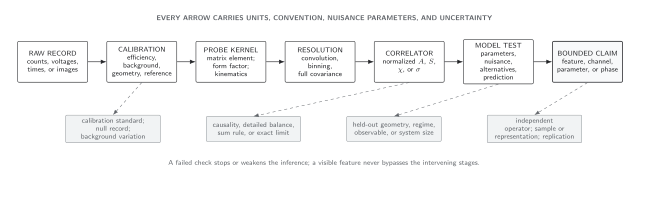
STM and QPI within the common forward map. Constant-current normalization, the tunneling orbital, surface termination, impurity potential, and instrumental resolution remain part of the conclusion. Schematic.

Quasiparticle interference is a response function

Let a defect have $T$ matrix $T(\omega)$. In a translationally invariant reference system, the Fourier component of the impurity-induced local density of states is schematically

$$\delta\rho(\mathbf q,\omega) =-\frac{1}{\pi}\operatorname{Im} \sum_{\mathbf k} \operatorname{Tr}\!\left[ P_eG_0^R(\mathbf k,\omega) T^R_{\mathbf k,\mathbf k+\mathbf q}(\omega) G_0^R(\mathbf k+\mathbf q,\omega) \right],$$

where $P_e$ projects onto the electron block in Nambu space. Peaks arise where spectral weight, group velocities, coherence factors, impurity selection rules, and joint phase space reinforce one another. Replacing this expression by an autocorrelation of $A(\mathbf k,\omega)$ discards the complex Green-function phase and $T$ matrix; it can suggest candidate wavevectors but cannot reproduce every intensity or absence.

In a superconductor, scalar, magnetic, pairing-amplitude, and orbital defects have different Nambu vertices. Their coherence factors can suppress a geometrically available scattering vector. Wang and Lee 2003 develop this Nambu-space QPI structure. A field-dependent QPI change may arise from vortices or magnetic scattering, but assigning a gap sign requires a model of those vertices, domains, impurity populations, and tunneling filters.

Calibration and negative tests

An accepted QPI analysis preserves the complex Fourier transform or explicitly states when only its modulus is used; treats windowing and drift correction; varies field of view; removes Bragg leakage without erasing nearby signal; checks multiple defects and terminations; propagates set-point and registration uncertainty; and compares simulated data after the same spatial mask and resolution. Three-dimensional band dispersion adds a surface-projection ambiguity quantified by Rhodes et al. 2023.

A hard gap requires vanishing low-energy spectral weight within a quantified noise floor and temperature broadening, not merely a V-shaped conductance. A bound state requires spatial localization and reproducible particle–hole structure, not one zero-bias pixel. A dispersing QPI branch constrains scattering geometry; it does not alone establish quasiparticle residue, bulk topology, or a pairing mechanism. The probe and computation claim test matrix records these distinctions.

Exercise

Thermal broadening. In the constant-tip limit, show that the conductance is a thermal convolution of the sample density of states rather than its exact value at $eV$.

Solution

Differentiate the tunneling current while taking $T$ and $\rho_t$ constant. After shifting variables,

$$\frac{dI}{dV}(V)\propto \int d\omega\,\rho_s(\omega) \left[-\frac{\partial f(\omega-eV)}{\partial\omega}\right].$$

The kernel $-f'$ is positive, integrates to one, and has width of order $k_BT$. Only as $T\to0$ does it approach $\delta(\omega-eV)$ and recover $\rho_s(eV)$ before instrumental voltage broadening is included.

References

• John Bardeen, “Tunnelling from a Many-Particle Point of View,” Physical Review Letters 6 (1961) 57–59. DOI
• Luke C. Rhodes, Weronika Osmolska, Carolina A. Marques, and Peter Wahl, “Nature of Quasiparticle Interference in Three Dimensions,” Physical Review B 107 (2023) 045107. DOI
• J. Tersoff and D. R. Hamann, “Theory and Application for the Scanning Tunneling Microscope,” Physical Review Letters 50 (1983) 1998–2001. DOI
• Qiang-Hua Wang and Dung-Hai Lee, “Quasiparticle Scattering Interference in High-Temperature Superconductors,” Physical Review B 67 (2003) 020511(R). DOI