BCS Mean-Field Theory and the Gap Equation

BCS mean-field theory turns an attractive Cooper channel into a self-consistent paired saddle. For a uniform, balanced, two-component system, the saddle produces particle–hole-mixed quasiparticles with $E_{\mathbf k}=\sqrt{\xi_{\mathbf k}^2+\lvert\Delta\rvert^2}$, coherence factors, and coupled gap and number equations. In the instantaneous isotropic weak-coupling model it also gives $2\Delta_0/T_c=2\pi \mathrm e^{-\gamma}\simeq3.53$. This page derives those results and their thermodynamics while keeping two ultraviolet completions distinct: a reduced-shell BCS model and a three-dimensional zero-range Fermi gas. Neither saddle identifies the pairing mediator, proves phase stiffness, nor becomes exact merely because it has a nonzero gap.

Required background. The Cooper instability supplies the attractive eigenchannel. Hubbard–Stratonovich fields supply the pairing-channel transformation.

Helpful background. Thermal effective potentials supply the saddle-point thermodynamic logic.

Two BCS models and one saddle

The algebra below is shared, but the parameters called “the interaction” and “the cutoff” are not interchangeable.

Ingredient	Reduced-shell model	Three-dimensional zero-range gas
Interaction data	An effective instantaneous attraction $-g$ retained in a shell $\lvert\xi\rvert<\omega_c$	A cutoff-dependent bare $g(\Lambda)$ matched to the physical scattering length $a$
Ultraviolet prescription	Keep $\omega_c$ as part of the model	Remove $\Lambda$ after subtracting the vacuum two-body divergence
Common ensemble	Often fixed $\mu$, with a particle–hole-symmetric density of states	Usually fixed total density $n$, so the gap and number equations are solved together
Weak-coupling statement	$N(0)g\ll1$ controls the reduced model	$k_Fa\to0^-$ controls the leading exponential, while medium effects change the mean-field prefactor

In both columns, let $\varepsilon_{\mathbf k}=\varepsilon_{-\mathbf k}$, $\xi_{\mathbf k}=\varepsilon_{\mathbf k}-\mu$, and

$$\int_{\mathbf k}\equiv\int\frac{\mathrm d^d k}{(2\pi)^d}, \qquad f(E)=\frac{1}{\mathrm e^{E/T}+1}.$$

The density $n$ below counts both fermion species. Whenever $N(0)$ is used, it is the normal-state density of states of one species at the Fermi surface. These declarations fix the factors of two that otherwise tend to migrate between the gap equation, the heat capacity, and the Nambu trace.

The two-state Nambu block also assumes that the proposed partners are degenerate before pairing,

$$\xi_{\mathbf k\uparrow}=\xi_{-\mathbf k\downarrow}\equiv\xi_{\mathbf k}.$$

Balance together with time-reversal or inversion symmetry supplies this relation in the models used here. With mismatch, define $\bar\xi=(\xi_{\mathbf k\uparrow}+\xi_{-\mathbf k\downarrow})/2$ and $\delta\xi=(\xi_{\mathbf k\uparrow}-\xi_{-\mathbf k\downarrow})/2$; the poles become $\delta\xi\pm\sqrt{\bar\xi^2+\lvert\Delta\rvert^2}$, so the formulas below cannot simply be reused.

Pairing-field saddle from the attractive interaction

For volume $\mathcal V$, collect zero-total-momentum pairs into

$$B=\sum_{\mathbf k}c_{-\mathbf k\downarrow}c_{\mathbf k\uparrow}, \qquad K_{\mathrm{int}}=-\frac{g}{\mathcal V}B^\dagger B, \qquad g>0.$$

Choose the pairing-field convention

$$\Delta=-\frac{g}{\mathcal V}\langle B\rangle =-g\int_{\mathbf k} \langle c_{-\mathbf k\downarrow}c_{\mathbf k\uparrow}\rangle.$$

Writing $B=\langle B\rangle+\delta B$ and dropping the quadratic fluctuation $\delta B^\dagger\delta B$ gives

$$K_{\mathrm{int}} \longrightarrow \Delta B^\dagger+\Delta^*B +\frac{\mathcal V\lvert\Delta\rvert^2}{g}.$$

The sign in the definition of $\Delta$ is conventional, but it must travel with the off-diagonal Nambu entries and the anomalous expectation value. In the basis

$$\Psi_{\mathbf k} =\begin{pmatrix}c_{\mathbf k\uparrow}\\ c^\dagger_{-\mathbf k\downarrow}\end{pmatrix},$$

the resulting mean-field grand-canonical Hamiltonian is

$$K_{\mathrm{MF}} =\sum_{\mathbf k}\Psi_{\mathbf k}^\dagger h_{\mathbf k}\Psi_{\mathbf k} +\sum_{\mathbf k}\xi_{\mathbf k} +\frac{\mathcal V\lvert\Delta\rvert^2}{g},$$

with

$$\begin{aligned} h_{\mathbf k} &=\xi_{\mathbf k}\tau_3 +\operatorname{Re}\Delta\,\tau_1 -\operatorname{Im}\Delta\,\tau_2,\\ \mathcal G^{-1}(\mathbf k,i\omega_n) &=i\omega_n\tau_0-h_{\mathbf k}\\ &=i\omega_n\tau_0-\xi_{\mathbf k}\tau_3 -\operatorname{Re}\Delta\,\tau_1 +\operatorname{Im}\Delta\,\tau_2. \end{aligned}$$

Thus the definition, mean-field decoupling, and inverse propagator form one sign-consistent chain. A common phase rotation can make a uniform one-component $\Delta$ real and positive for the diagonalization; this is a basis choice, not a new observable.

Nambu spectrum, coherence factors, and the paired state

The determinant

$$\det\mathcal G^{-1}(\mathbf k,i\omega_n) =(i\omega_n)^2-\xi_{\mathbf k}^2-\lvert\Delta\rvert^2$$

has particle–hole-related poles at $\pm E_{\mathbf k}$, where

$$E_{\mathbf k}=\sqrt{\xi_{\mathbf k}^2+\lvert\Delta\rvert^2}.$$

For real $\Delta>0$, a positive-energy eigenvector of $h_{\mathbf k}$ may be chosen with nonnegative entries $(u_{\mathbf k},v_{\mathbf k})^T$. The eigenvalue equation and normalization give

$$\begin{aligned} u_{\mathbf k}^2 &=\frac12\left(1+\frac{\xi_{\mathbf k}}{E_{\mathbf k}}\right), & v_{\mathbf k}^2 &=\frac12\left(1-\frac{\xi_{\mathbf k}}{E_{\mathbf k}}\right),\\ u_{\mathbf k}^2-v_{\mathbf k}^2 &=\frac{\xi_{\mathbf k}}{E_{\mathbf k}}, & 2u_{\mathbf k}v_{\mathbf k} &=\frac{\Delta}{E_{\mathbf k}}. \end{aligned}$$

Far above the Fermi surface the positive branch is particle-like, $u^2\to1$; far below it is hole-like, $v^2\to1$. If the accessible dispersion crosses $\xi_{\mathbf k}=0$, the two weights are equal there and the minimum positive excitation is $\Delta$. The separation between the plotted partner branches at that crossing is $2\Delta$; calling that separation “the gap” without specifying the observable is a common factor-of-two error. If no allowed state has $\xi_{\mathbf k}=0$, the minimum moves to the band edge and need not equal $\Delta$; for $\varepsilon_k=k^2/(2m)$ with $\mu<0$, it is $\sqrt{\mu^2+\lvert\Delta\rvert^2}$ at $k=0$.

The dimensionless curves make both statements visible. Follow the solid paired branches away from the dashed normal crossing, then compare how the two coherence weights exchange through the Fermi surface.

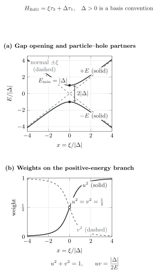
For a uniform BCS saddle whose normal-state dispersion crosses $\xi=0$, the Nambu branches $\pm\sqrt{\xi^2+\lvert\Delta\rvert^2}$ avoid the normal crossing. The minimum positive excitation is $\lvert\Delta\rvert$, while the partner-branch separation at $\xi=0$ is $2\lvert\Delta\rvert$. On the positive branch, the particle and hole weights interchange through $u^2=v^2=1/2$ while $u^2+v^2=1$. Exact dimensionless BCS curves, not material data.

Download the curves as SVG, inspect the numerical values, or read the semantic record.

At zero temperature, the same convention is represented by the product state

$$\lvert\mathrm{BCS}\rangle =\prod_{\mathbf k}^{\text{independent pairs}} \left( u_{\mathbf k} -v_{\mathbf k}c^\dagger_{\mathbf k\uparrow} c^\dagger_{-\mathbf k\downarrow} \right)\lvert0\rangle.$$

It has $\langle c_{-\mathbf k\downarrow}c_{\mathbf k\uparrow}\rangle=-u_{\mathbf k}v_{\mathbf k}$. At finite temperature this becomes

$$\langle c_{-\mathbf k\downarrow}c_{\mathbf k\uparrow}\rangle =-\frac{\Delta}{2E_{\mathbf k}} \tanh\frac{E_{\mathbf k}}{2T},$$

which closes the self-consistency loop with the chosen definition of $\Delta$. Bardeen, Cooper, and Schrieffer 1957, §II, pp. 1179–1183 develop the paired state, excitation spectrum, and zero-temperature gap construction.

The eigenvalues $+E$ and $-E$ are partner labels in an enlarged particle–hole representation, not two independent orbitals. The reduced spin block above may be summed over every $\mathbf k$ with no extra $1/2$; its two spin-degenerate positive quasiparticles appear after the full Bogoliubov transformation. A fully doubled Nambu basis instead requires a factor $1/2$ in the quadratic form or an equivalent restriction. Remove the redundancy exactly once.

Grand potential, gap equation, and number equation

The fermion trace gives the cutoff grand-potential density

$$\frac{\Omega(\Delta,\mu,T)}{\mathcal V} =\frac{\lvert\Delta\rvert^2}{g} +\int_{\mathbf k}(\xi_{\mathbf k}-E_{\mathbf k}) -2T\int_{\mathbf k}\log\!\left(1+\mathrm e^{-E_{\mathbf k}/T}\right).$$

The first term is the pairing-field cost. The zero-point term $\xi-E$ restores the normal-ordering constant introduced by the Nambu basis, and the factor $2$ in the thermal term counts the two spin-degenerate positive quasiparticles. Setting $\Delta=0$ recovers the grand potential of two free fermion species.

Stationarity with respect to the complex field gives

$$\frac{1}{\mathcal V}\frac{\partial\Omega}{\partial\Delta^*} =\Delta\left[ \frac1g -\int_{\mathbf k} \frac{1-2f(E_{\mathbf k})}{2E_{\mathbf k}} \right].$$

The normal solution $\Delta=0$ is always stationary. A nonzero saddle therefore obeys

$$\frac1g =\int_{\mathbf k} \frac{1-2f(E_{\mathbf k})}{2E_{\mathbf k}} =\int_{\mathbf k} \frac{\tanh(E_{\mathbf k}/2T)}{2E_{\mathbf k}}.$$

At fixed total density, use the saddle-point identity

$$n=-\frac1{\mathcal V} \frac{\mathrm d\Omega(\Delta_{\mathrm{sp}}(\mu),\mu,T)}{\mathrm d\mu} =-\frac1{\mathcal V} \frac{\partial\Omega}{\partial\mu},$$

because $\partial\Omega/\partial\Delta=0$ removes the implicit derivative of the saddle. The number equation is

$$n=\int_{\mathbf k} \left[ 1-\frac{\xi_{\mathbf k}}{E_{\mathbf k}} \bigl(1-2f(E_{\mathbf k})\bigr) \right].$$

As $\Delta\to0$, its integrand reduces to $2f(\xi_{\mathbf k})$, an immediate check on the spin factor. At fixed $\mu$, only the gap equation is needed. At fixed $n$, the gap and number equations determine $\Delta$ and $\mu$ together; inserting the normal-state chemical potential by hand generally violates the declared ensemble.

Ultraviolet matching for the contact gas

For a uniform, balanced, equal-mass, broad-resonance, zero-effective-range continuum saddle in three dimensions, take $\varepsilon_{\mathbf k}=k^2/(2m)$. The vacuum scattering amplitude relates the cutoff bare coupling to the physical scattering length:

$$\frac{1}{g(\Lambda)} =-\frac{m}{4\pi a} +\int_{\mathbf k}^{\Lambda}\frac{1}{2\varepsilon_{\mathbf k}}.$$

Substituting before removing $\Lambda$ gives the finite grand potential

$$\begin{aligned} \frac{\Omega_{\mathrm R}}{\mathcal V} ={}&-\frac{m\lvert\Delta\rvert^2}{4\pi a}\\ &+\int_{\mathbf k} \left( \xi_{\mathbf k}-E_{\mathbf k} +\frac{\lvert\Delta\rvert^2}{2\varepsilon_{\mathbf k}} \right)\\ &-2T\int_{\mathbf k} \log\!\left(1+\mathrm e^{-E_{\mathbf k}/T}\right). \end{aligned}$$

Its stationarity condition is

$$-\frac{m}{4\pi a} =\int_{\mathbf k}\left[ \frac{1-2f(E_{\mathbf k})}{2E_{\mathbf k}} -\frac{1}{2\varepsilon_{\mathbf k}} \right].$$

At large momentum, the two terms in the brackets cancel at order $1/k^2$, leaving an integrable $1/k^4$ tail. The corresponding subtraction in $\Omega_{\mathrm R}$ is equally necessary: renormalizing only the gap equation while evaluating the bare grand potential is inconsistent. This zero-range form also assumes the effective range and other microscopic lengths are negligible on the many-body scale. The pairing-only saddle omits a normal-state Hartree or Fermi-liquid self-energy; such a term must either be absorbed consistently into $\xi_{\mathbf k}$ or computed beyond this approximation.

The contact-interaction page derives the two-body matching. Leggett 1980, pp. 13–27 follows the same variational state from overlapping Cooper pairs toward diatomic molecules. Sá de Melo, Randeria, and Engelbrecht 1993, pp. 3202–3204 and Giorgini, Pitaevskii, and Stringari 2008, §V.A, p. 1229, Eqs. (54)–(56) develop the regulated gap-and-number saddle and its limitations across coupling.

Reduced-shell weak-coupling solution

Now switch deliberately to the first column of the model table. Assume an instantaneous isotropic attraction, a symmetric shell $\lvert\xi\rvert<\omega_c$, a smooth nonzero single-spin density of states approximated by $N(0)$, and $N(0)g\ll1$ with $T_c,\Delta_0\ll\omega_c$. At $T=0$,

$$\begin{aligned} \frac{1}{N(0)g} &=\int_0^{\omega_c} \frac{\mathrm d\xi}{\sqrt{\xi^2+\Delta_0^2}}\\ &=\operatorname{arsinh}\frac{\omega_c}{\Delta_0} =\log\frac{2\omega_c}{\Delta_0} +O\!\left(\frac{\Delta_0^2}{\omega_c^2}\right). \end{aligned}$$

Therefore

$$\Delta_0=2\omega_c\exp\!\left[-\frac{1}{N(0)g}\right]$$

to leading weak-coupling accuracy. At the transition, take $\Delta\to0$ in the same equation:

$$\begin{aligned} \frac{1}{N(0)g} &=\int_0^{\omega_c}\frac{\mathrm d\xi}{\xi} \tanh\frac{\xi}{2T_c}\\ &=\log\frac{2\mathrm e^\gamma\omega_c}{\pi T_c} +O\!\left(\mathrm e^{-\omega_c/T_c}\right). \end{aligned}$$

Eliminating the same $g$ and $\omega_c$ from the two equations gives

$$T_c=\frac{2\mathrm e^\gamma}{\pi}\omega_c \exp\!\left[-\frac{1}{N(0)g}\right], \qquad \frac{2\Delta_0}{T_c}=\frac{2\pi}{\mathrm e^\gamma}\simeq3.53.$$

The pure number is universal only inside this instantaneous, isotropic, weak-coupling model. An energy-dependent density of states or cutoff, gap anisotropy, pair breaking, and finite-coupling retarded or strong-coupling effects can change it; the weak-coupling retarded limit tends back to the BCS value. A band edge, van Hove singularity, or vanishing density of states can also invalidate the exponential solution itself. Bardeen, Cooper, and Schrieffer 1957, §III, p. 1186, Eqs. (3.27)–(3.30) set up the finite-temperature construction and report its original numerical approximations; the exact constant above follows from the convergent integral just evaluated.

For comparison, the zero-range contact saddle at $k_Fa\to0^-$ gives

$$\Delta_0^{\mathrm{MF}} =\frac{8}{\mathrm e^2}E_F \exp\!\left(\frac{\pi}{2k_Fa}\right).$$

This shares the BCS exponential but not the shell model’s cutoff. Particle–hole screening changes both $\Delta_0$ and $T_c$ by the finite factor

$$\frac{\Delta_0^{\mathrm{GMB}}}{\Delta_0^{\mathrm{MF}}} =\frac{T_c^{\mathrm{GMB}}}{T_c^{\mathrm{MF}}} =(4\mathrm e)^{-1/3}\simeq0.45$$

even as $k_F\lvert a\rvert\to0$. Thus weak coupling controls the leading logarithm and makes the critical fluctuation region narrow, but it does not make the bare pairing saddle’s prefactor exact. Gor’kov and Melik-Barkhudarov 1961, pp. 1021–1022 give the medium correction; Giorgini, Pitaevskii, and Stringari 2008, §IV.D, p. 1225, Eqs. (33)–(35) translate it into the dilute-gas convention.

Thermodynamic checks

At $T=0$ and the same chemical potential, subtract the normal grand potential in the symmetric shell:

$$\begin{aligned} \frac{\Omega_s-\Omega_n}{\mathcal V} ={}&\frac{\Delta_0^2}{g} +2N(0)\int_0^{\omega_c}\mathrm d\xi \left(\xi-\sqrt{\xi^2+\Delta_0^2}\right)\\ ={}&N(0)\omega_c \left(\omega_c-\sqrt{\omega_c^2+\Delta_0^2}\right)\\ ={}&-\frac12N(0)\Delta_0^2 +O\!\left(\frac{N(0)\Delta_0^4}{\omega_c^2}\right). \end{aligned}$$

The gap equation performs the cancellation that leaves the negative condensation energy. At fixed density the comparison is instead between Helmholtz free energies $F_s$ and $F_n$ after adjusting each chemical potential. The same leading coefficient follows in the particle–hole-symmetric weak-coupling limit, but it is not an exact ensemble identity.

Near $T_c$, expanding the same grand potential gives

$$\frac{\Omega(\Delta)-\Omega_n}{\mathcal V} =N(0)\frac{T-T_c}{T_c}\lvert\Delta\rvert^2 +\frac{7\zeta(3)N(0)}{16\pi^2T_c^2}\lvert\Delta\rvert^4 +O\!\left(\frac{N(0)\lvert\Delta\rvert^6}{T_c^4}\right).$$

Minimization yields

$$\lvert\Delta(T)\rvert^2 =\frac{8\pi^2T_c^2}{7\zeta(3)} \left(1-\frac{T}{T_c}\right)$$

just below $T_c$. With normal-state heat-capacity density $c_n=\gamma_nT$ and $\gamma_n=2\pi^2N(0)/3$ for the two spin species,

$$\frac{\Delta c}{\gamma_nT_c} =\frac{c_s(T_c^-)-c_n(T_c^+)}{\gamma_nT_c} =\frac{12}{7\zeta(3)}\simeq1.43.$$

The displayed expansion and jump are fixed-$\mu$ statements. At fixed density one must Legendre-transform and include the temperature-dependent chemical-potential shift; the same leading jump follows in the symmetric constant-density-of-states approximation used here, not as a general ensemble identity. The $\zeta(3)$ coefficient is the uniform part of the microscopic Ginzburg–Landau expansion derived in Gor’kov 1959, pp. 1365–1366. The condensation energy, gap ratio, and heat-capacity jump form a mutually consistent check of the same density-of-states convention. They are predictions of the reduced model, not universal material diagnostics or evidence for a specific mediator.

What the saddle establishes—and what it does not

A solution of the gap and number equations establishes a stationary paired propagator for the declared model. It must still be compared with the normal state and any competing saddles, and its amplitude Hessian must be nonnegative. A negative eigenvalue of the fluctuation kernel means the proposed saddle is not the equilibrium state, while the phase direction of a neutral broken-symmetry saddle becomes a collective coordinate rather than an ordinary massive fluctuation. In imbalanced or multichannel extensions, a nonzero solution can therefore be unstable.

In a finite neutral system with exact particle number, $\langle cc\rangle$ vanishes. The thermodynamic broken-symmetry construction is understood through a quasiaverage or, equivalently, off-diagonal long-range order in a number-conserving description; Yang 1962, pp. 694–704 formulates the latter criterion. In a charged theory, $\Delta$ is gauge covariant and a chosen phase is gauge-fixed; local gauge redundancy is not itself a broken observable symmetry, as emphasized by Elitzur 1975, pp. 3978–3982. Spectra, free-energy derivatives, phase stiffness, and gauge-invariant response carry the physical conclusions.

The thermal critical region of a clean three-dimensional weak-coupling BCS system is parametrically narrow when $T_c/E_F\ll1$, but this does not suppress the induced-interaction correction above or license mean field in low dimension; Larkin and Varlamov 2001, §2.2 separates the Ginzburg criterion from these other corrections. In two dimensions, a nonzero saddle can mark pair formation while the actual finite-temperature coherence transition is controlled by phase stiffness and vortex unbinding, the mechanism identified in Kosterlitz and Thouless 1973, pp. 1181–1203. At strong coupling, low density, strong disorder, imbalance, or without a clean scale separation, amplitude, number, and phase fluctuations require separate control.

The structure diagram shows where the saddle sits in the longer chain. Inspect the branches after “paired saddle”: none follows from the gap equation without additional input.

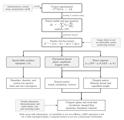
BCS self-consistency fixes a paired saddle and its quasiparticle spectrum. It does not by itself establish phase rigidity, Meissner screening, a microscopic mechanism, or topology. Original schematic, not to scale.

Download the structure map as SVG, inspect its machine-readable relations, and use the paired-matter claim test matrix to identify the control and negative test for each stronger claim.

Common pitfalls

Changing one sign in isolation. Rephasing a Nambu component or redefining $\Delta$ can reverse off-diagonal signs without changing observables. The definition of $\Delta$, mean-field Hamiltonian, anomalous average, and coherence-factor phase must all transform together.

Counting the Nambu partners twice. The $\pm E$ eigenvalues encode particle–hole redundancy. Use a reduced spin block over all momenta or a fully doubled basis with a factor $1/2$—not both corrections and not neither.

Losing the density-of-states convention. Here $N(0)$ is per spin, whereas $\gamma_n$ includes both spins. Substituting a spin-summed density of states into only one formula changes the condensation energy or heat jump by two.

Mixing the two ultraviolet models. The shell cutoff $\omega_c$ is retained physical input to a reduced model; the contact cutoff $\Lambda$ must disappear in favor of $a$. Combining $\omega_c$ and $a$ in one gap equation without a matching calculation defines neither model.

Confusing fixed $\mu$ with fixed $n$. The gap equation alone extremizes the grand potential at fixed chemical potential. A density-controlled problem also requires the number equation, and phase comparisons use $F$, not $\Omega$, after the chemical potentials are adjusted.

Promoting a gap into a stronger claim. A nonzero $\Delta$, the ratio $3.53$, or the jump $1.43$ does not by itself establish phase stiffness, Meissner screening, a microscopic mechanism, or quantitative validity at strong coupling.

Exercises

Close the sign round trip

Starting from $K_{\mathrm{int}}=-(g/\mathcal V)B^\dagger B$ and $\Delta=-(g/\mathcal V)\langle B\rangle$, reproduce the mean-field interaction and show that the upper-right entry of $h_{\mathbf k}$ is $+\Delta$.

Solution

Keeping only terms linear in $\delta B=B-\langle B\rangle$ gives

$$B^\dagger B \simeq \langle B^\dagger\rangle B +B^\dagger\langle B\rangle -\langle B^\dagger\rangle\langle B\rangle.$$

Since $\langle B\rangle=-\mathcal V\Delta/g$, multiplication by $-g/\mathcal V$ yields

$$K_{\mathrm{int}}^{\mathrm{MF}} =\Delta^*B+\Delta B^\dagger +\frac{\mathcal V\lvert\Delta\rvert^2}{g}.$$

The term $\Delta c^\dagger_{\mathbf k\uparrow}c^\dagger_{-\mathbf k\downarrow}$ is the upper-right entry of $\Psi_{\mathbf k}^\dagger h_{\mathbf k}\Psi_{\mathbf k}$, so

$$h_{\mathbf k} =\begin{pmatrix} \xi_{\mathbf k}&\Delta\\ \Delta^*&-\xi_{\mathbf k} \end{pmatrix}.$$

Consequently $\mathcal G^{-1}=i\omega_n-h$ has upper-right entry $-\Delta$. A redefinition $\Delta\mapsto-\Delta$ is harmless only if it is applied to every line in this chain.

Diagonalize and count once

For real $\Delta>0$, diagonalize $h=\xi\tau_3+\Delta\tau_1$. Derive the four coherence-factor identities above. When the allowed dispersion includes $\xi=0$, identify the minimum positive excitation and the partner-branch separation, and explain what would be doubled by summing both Nambu eigenvalues as independent excitations.

Solution

The characteristic polynomial is $E^2-\xi^2-\Delta^2$, so the eigenvalues are $\pm E$ with $E=\sqrt{\xi^2+\Delta^2}$. For the positive eigenvector,

$$(E-\xi)u=\Delta v, \qquad u^2+v^2=1.$$

Solving gives

$$u^2=\frac12\left(1+\frac{\xi}{E}\right), \qquad v^2=\frac12\left(1-\frac{\xi}{E}\right),$$

and subtraction and multiplication give $u^2-v^2=\xi/E$ and $2uv=\Delta/E$. Provided an allowed momentum has $\xi=0$, the minimum of $E$ is $\Delta$ there, while the distance from $-E$ to $+E$ is $2\Delta$. If the spectrum never reaches $\xi=0$, one must instead minimize $E_{\mathbf k}$ over its physical momentum domain. Treating both signs as independent positive-energy states would double the particle–hole representation; physical spin degeneracy is counted separately by the two Bogoliubov quasiparticles.

Differentiate the grand potential

Derive the gap and number equations from $\Omega$. Then take $\Delta\to0$ in the number equation and recover the density of two free species.

Solution

Using $\partial E/\partial\Delta^*=\Delta/(2E)$ and $\mathrm d\log(1+\mathrm e^{-E/T})/\mathrm dE=-f(E)/T$ gives

$$\frac1{\mathcal V}\frac{\partial\Omega}{\partial\Delta^*} =\Delta\left[ \frac1g-\int_{\mathbf k}\frac{1-2f(E)}{2E} \right].$$

For the number derivative, $\partial\xi/\partial\mu=-1$ and $\partial E/\partial\mu=-\xi/E$. At the saddle the chain-rule term proportional to $\mathrm d\Delta_{\mathrm{sp}}/\mathrm d\mu$ vanishes, leaving

$$n=\int_{\mathbf k}\left[ 1-\frac{\xi}{E}(1-2f(E)) \right].$$

When $\Delta=0$, $E=\lvert\xi\rvert$. For $\xi>0$ the integrand is $2f(\xi)$; for $\xi<0$, use $f(-\lvert\xi\rvert)=1-f(\lvert\xi\rvert)$ to obtain the same expression. Hence $n=2\int_{\mathbf k}f(\xi_{\mathbf k})$.

Make the contact equation finite

Insert the scattering-length matching relation into the bare gap equation and grand potential. Show from the large-$k$ expansion that both resulting integrals converge in three dimensions.

Solution

Replacing $1/g(\Lambda)$ in the gap equation and moving the vacuum term to the integrand gives

$$-\frac{m}{4\pi a} =\int_{\mathbf k}\left[ \frac{1-2f(E)}{2E}-\frac{1}{2\varepsilon} \right].$$

For $k\to\infty$, thermal occupation is exponentially small and

$$E=\xi+\frac{\lvert\Delta\rvert^2}{2\xi}+O(k^{-6}), \qquad \xi=\varepsilon-\mu.$$

Therefore $1/(2E)-1/(2\varepsilon)=O(k^{-4})$. With the three-dimensional measure $k^2\mathrm dk$, the tail behaves as $\mathrm dk/k^2$ and converges. In the grand potential, the combination $\xi-E+\lvert\Delta\rvert^2/(2\varepsilon)$ also begins at $O(k^{-4})$. The same vacuum subtraction is required in both quantities.

Obtain the weak-coupling ratio

Evaluate the zero-temperature shell integral and linearize the finite-temperature equation at $T_c$. Eliminate $N(0)g$ and $\omega_c$ to obtain $2\Delta_0/T_c$.

Solution

At $T=0$,

$$\frac1{N(0)g} =\operatorname{arsinh}\frac{\omega_c}{\Delta_0} \simeq\log\frac{2\omega_c}{\Delta_0}.$$

At $T_c$, substitute $x=\xi/(2T_c)$ and use the large-$A$ identity

$$\int_0^A\frac{\tanh x}{x}\,\mathrm dx =\log\frac{4\mathrm e^\gamma A}{\pi}+O(\mathrm e^{-2A}).$$

This gives

$$\frac1{N(0)g} =\log\frac{2\mathrm e^\gamma\omega_c}{\pi T_c}.$$

Equating the two logarithms yields $\Delta_0/T_c=\pi/\mathrm e^\gamma$, hence $2\Delta_0/T_c=2\pi/\mathrm e^\gamma\simeq3.53$. The cancellation works only because both equations use the same instantaneous interaction, cutoff, density of states, and weak-coupling approximation.

Separate ensemble from claim

Use the zero-temperature shell grand potential and the gap equation to obtain the leading same-$\mu$ condensation energy. Then state which additional calculations are needed before claiming a neutral superfluid, a charged superconductor, or a microscopic pairing mechanism.

Solution

Subtracting the normal state gives

$$\frac{\delta\Omega}{\mathcal V} =\frac{\Delta_0^2}{g} +2N(0)\int_0^{\omega_c}\mathrm d\xi \left(\xi-\sqrt{\xi^2+\Delta_0^2}\right).$$

Using the exact shell gap equation before expanding cancels the inverse-hyperbolic-sine terms and gives

$$\frac{\delta\Omega}{\mathcal V} =N(0)\omega_c \left(\omega_c-\sqrt{\omega_c^2+\Delta_0^2}\right) =-\frac12N(0)\Delta_0^2 +O\!\left(\frac{N(0)\Delta_0^4}{\omega_c^2}\right).$$

At fixed $n$, compare $F=\Omega+\mu N$ after solving the number equation in each phase. A neutral-superfluid claim additionally needs phase stiffness or an equivalent coherence diagnostic. A charged-superconductor claim needs gauge-invariant electromagnetic response, including the diamagnetic term and Ward consistency. A mechanism claim needs a controlled microscopic interaction and competing-channel analysis; none follows from the stationary gap alone.

Continue

Nambu–Gor’kov propagators develop anomalous Green functions, basis translations, and particle–hole redundancy beyond this uniform saddle. The BCS–BEC crossover solves the regulated contact equations away from weak coupling and shows where mean field fails quantitatively. Phase stiffness and vortices determine whether pairing acquires long-range or topological phase coherence. Migdal control and Eliashberg theory replace the instantaneous shell interaction by a retarded kernel.

References

• Bardeen, J., Cooper, L. N., and Schrieffer, J. R. (1957). “Theory of superconductivity.” Physical Review 108, 1175–1204. doi:10.1103/PhysRev.108.1175.
• Elitzur, S. (1975). “Impossibility of spontaneously breaking local symmetries.” Physical Review D 12, 3978–3982. doi:10.1103/PhysRevD.12.3978.
• Giorgini, S., Pitaevskii, L. P., and Stringari, S. (2008). “Theory of ultracold atomic Fermi gases.” Reviews of Modern Physics 80, 1215–1274. doi:10.1103/RevModPhys.80.1215.
• Gor’kov, L. P. (1959). “Microscopic derivation of the Ginzburg–Landau equations in the theory of superconductivity.” Soviet Physics JETP 9, 1364–1367. JETP archive PDF.
• Gor’kov, L. P., and Melik-Barkhudarov, T. K. (1961). “Contribution to the theory of superfluidity in an imperfect Fermi gas.” Soviet Physics JETP 13, 1018–1022. JETP archive PDF.
• Kosterlitz, J. M., and Thouless, D. J. (1973). “Ordering, metastability and phase transitions in two-dimensional systems.” Journal of Physics C: Solid State Physics 6, 1181–1203. doi:10.1088/0022-3719/6/7/010.
• Larkin, A., and Varlamov, A. (2001). “Fluctuation phenomena in superconductors.” arXiv:cond-mat/0109177. arXiv abstract.
• Leggett, A. J. (1980). “Diatomic molecules and Cooper pairs.” In A. Pękalski and J. A. Przystawa (eds.), Modern Trends in the Theory of Condensed Matter, Lecture Notes in Physics 115, pp. 13–27. Springer. doi:10.1007/BFb0120125.
• Sá de Melo, C. A. R., Randeria, M., and Engelbrecht, J. R. (1993). “Crossover from BCS to Bose superconductivity: Transition temperature and time-dependent Ginzburg–Landau theory.” Physical Review Letters 71, 3202–3205. doi:10.1103/PhysRevLett.71.3202.
• Yang, C. N. (1962). “Concept of off-diagonal long-range order and the quantum phases of liquid He and of superconductors.” Reviews of Modern Physics 34, 694–704. doi:10.1103/RevModPhys.34.694.