Topological BdG Superconductors and Boundary Modes

A topological Bogoliubov–de Gennes (BdG) Hamiltonian does not guarantee a Majorana mode by itself. The conclusion follows only after specifying the symmetry class, a gapped ultraviolet-complete bulk, and an interface or defect across which the relevant invariant changes. The Kitaev chain makes that logic calculable: its bulk invariant, normalized end-mode profile, localization length, and finite-size splitting can all be derived explicitly. We then use the same logic for two-dimensional chiral superconductors and semiconductor–superconductor wires, while keeping model predictions separate from device and non-Abelian claims.

Required background. Inhomogeneous BdG theory supplies Nambu redundancy, boundary conditions, and quasiparticle normalization.

Helpful background. The free-fermion periodic table and protected interfaces supply the classification and bulk–boundary framework.

The Kitaev chain as a BdG Hamiltonian

Consider an infinite or periodic chain of spinless fermions with real $t$ and $\Delta$:

$$H=\sum_j\left[ -t(c_j^\dagger c_{j+1}+c_{j+1}^\dagger c_j) -\mu\left(c_j^\dagger c_j-\frac12\right) +\Delta(c_jc_{j+1}+c_{j+1}^\dagger c_j^\dagger) \right].$$

Use $c_j=L^{-1/2}\sum_k e^{ikj}c_k$ and the Nambu spinor $\Psi_k=(c_k,c_{-k}^\dagger)^T$. Summing over the full Brillouin zone doubles the Nambu description, so the factor $1/2$ is essential:

$$H=\frac12\sum_k\Psi_k^\dagger\mathcal H(k)\Psi_k+\text{constant}, \qquad \mathcal H(k)=d_z(k)\tau_z+d_y(k)\tau_y,$$ $$d_z(k)=-\mu-2t\cos k, \qquad d_y(k)=2\Delta\sin k.$$

The intrinsic BdG particle–hole operation is

$$\mathcal C=\tau_xK, \qquad \mathcal C^2=+1, \qquad \mathcal C\mathcal H(k)\mathcal C^{-1}=-\mathcal H(-k).$$

It expresses Nambu redundancy, not an independently imposed microscopic symmetry: an eigenvector at $(k,E)$ has a redundant partner at $(-k,-E)$. The two eigenvalues are

$$E_\pm(k)=\pm\sqrt{(\mu+2t\cos k)^2+4\Delta^2\sin^2k}.$$

For $\Delta\ne0$, both terms can vanish only at

$$(k,\mu)=(0,-2t) \quad\text{or}\quad (k,\mu)=(\pi,2t).$$

Thus $\lvert\mu\rvert<2\lvert t\rvert$ and $\lvert\mu\rvert>2\lvert t\rvert$ are distinct gapped phases. At the line $t=\Delta>0$, the bulk gap is especially transparent:

$$E_{\mathrm{gap}}=\min_k\lvert E_\pm(k)\rvert =\bigl\lvert\,\lvert\mu\rvert-2t\,\bigr\rvert.$$

Because all coefficients are real, this representative also obeys spinless time reversal $\mathcal T=K$, with $\mathcal T^2=+1$, and chiral symmetry $\mathcal S=\mathcal T\mathcal C=\tau_x$. It is therefore in class BDI. In a basis that diagonalizes $\mathcal S$, the off-diagonal function can be taken as

$$q(k)=d_z(k)+i\,d_y(k), \qquad w=\frac{1}{2\pi i}\int_{-\pi}^{\pi}dk\, \partial_k\log q(k).$$

As $k$ crosses the Brillouin zone, $q(k)$ traces an ellipse centered at $-\mu$. The ellipse encloses the origin precisely when $\lvert\mu\rvert<2\lvert t\rvert$, giving $\lvert w\rvert=1$; the sign of $w$ depends on the orientation conventions for the chain and pairing. A uniform global phase of $\Delta$ is removable by a Nambu gauge rotation and therefore does not by itself break the spinless time-reversal structure. Gauge-invariant complex structure—such as relative pairing phases, supercurrent, or flux—breaks $\mathcal T$ and $\mathcal S$ while preserving $\mathcal C$, reducing the problem to class D, where only $w\bmod 2$ survives.

At the particle–hole-invariant momenta $k=0,\pi$, the matrix $B(k)=\mathcal H(k)\tau_x$ is antisymmetric. With one continuous, consistently oriented Majorana basis,

$$\operatorname{Pf}B(0)=-\mu-2t, \qquad \operatorname{Pf}B(\pi)=-\mu+2t,$$

and the class-D parity is

$$\mathcal M =\operatorname{sgn}\!\left[ \operatorname{Pf}B(0)\operatorname{Pf}B(\pi) \right] =\operatorname{sgn}\!\left[(-\mu-2t)(-\mu+2t)\right].$$

$\mathcal M=-1$ is the nontrivial phase. An orientation-reversing basis change flips an individual Pfaffian, so signs computed in unrelated gauges must not be compared. The product is invariant when the same continuous orientation is used at both momenta, and it is undefined at either bulk closing. Kitaev 2001, §§2–3 gives the Majorana-number construction and its boundary-parity consequence.

The open-chain Majorana solution

Now cut the chain after $L$ sites and define Hermitian Majorana operators

$$a_j=c_j+c_j^\dagger, \qquad b_j=-i(c_j-c_j^\dagger), \qquad \{a_i,a_j\}=\{b_i,b_j\}=2\delta_{ij}.$$

The open-chain Hamiltonian becomes

$$\begin{aligned} H={}&\frac{i}{2}\sum_{j=1}^{L}(-\mu\,a_jb_j)\\ &+\frac{i}{2}\sum_{j=1}^{L-1} \left[(t+\Delta)b_ja_{j+1}+(\Delta-t)a_jb_{j+1}\right]. \end{aligned}$$

Equivalently, $H=(i/4)\boldsymbol\gamma^TA\boldsymbol\gamma$ for a real antisymmetric Majorana matrix $A$. Seek a left mode $\Gamma_L=\sum_{j=1}^L\alpha_j a_j$. The interior zero-mode equation $A\boldsymbol v_L=0$ is

$$(t+\Delta)\alpha_{j+1} +\mu\alpha_j +(t-\Delta)\alpha_{j-1}=0, \qquad \alpha_0=0.$$

For $t+\Delta\ne0$, use $\alpha_j\propto\lambda^j$. The characteristic roots obey

$$(t+\Delta)\lambda^2+\mu\lambda+(t-\Delta)=0,$$ $$\lambda_\pm= \frac{-\mu\pm\sqrt{\mu^2-4(t^2-\Delta^2)}}{2(t+\Delta)}.$$

For distinct roots, the semi-infinite boundary condition selects $\alpha_j\propto\lambda_+^j-\lambda_-^j$. At the repeated-root discriminant $\mu^2=4(t^2-\Delta^2)$, its continuous limit is $\alpha_j\propto j\lambda^{j-1}$. A normalizable end state requires the selected root factors to lie inside the unit circle. Roots may be real or a complex-conjugate pair, so decay can be monotone or oscillatory. If $t+\Delta=0$, one instead solves the recurrence in the opposite direction or exchanges the two Majorana sublattices; it is not covered by the displayed root formula.

At $t=\Delta>0$, one root vanishes and the other is

$$r=-\frac{\mu}{2t}.$$

For $\lvert r\rvert<1$, finite-$L$-normalized profiles truncated from the two semi-infinite solutions are

$$\Gamma_L^{\mathrm{trial}} =\mathcal N_L\sum_{j=1}^{L}r^{j-1}a_j, \qquad \Gamma_R^{\mathrm{trial}} =\mathcal N_L\sum_{j=1}^{L}r^{L-j}b_j,$$ $$\mathcal N_L =\left(\sum_{j=0}^{L-1}r^{2j}\right)^{-1/2} =\sqrt{\frac{1-r^2}{1-r^{2L}}}.$$

This normalization gives $(\Gamma_{L,R}^{\mathrm{trial}})^2=1$. In the site-ordered Nambu coordinates $(u_1,\ldots,u_L,v_1,\ldots,v_L)^T$, the corresponding Euclidean unit vector is

$$\Phi_L =\frac{1}{\sqrt2} \begin{pmatrix} \boldsymbol\alpha\\ \boldsymbol\alpha \end{pmatrix}, \qquad \boldsymbol\alpha =\mathcal N_L(1,r,\ldots,r^{L-1})^T,$$ $$\Phi_L^\dagger\Phi_L=1, \qquad \mathcal C\Phi_L=\Phi_L.$$

The factor $1/\sqrt2$ reconciles two common conventions: $\Gamma_L^2=1$ for a Majorana operator with $\{\Gamma_L,\Gamma_L\}=2$, whereas a BdG quasiparticle vector has unit Euclidean norm.

For a semi-infinite chain, the recurrence is exact. On a finite chain, the truncated left profile fails only at the far boundary:

$$\lVert A\boldsymbol v_L\rVert =\lvert\mu\rvert\mathcal N_L\lvert r\rvert^{L-1} =2t\,\mathcal N_L\lvert r\rvert^L.$$

It is therefore an exact finite-chain zero mode only at $r=0$, or in the $L\to\infty$ limit. The amplitude obeys

$$\lvert\alpha_j\rvert\propto e^{-(j-1)a/\xi_M}, \qquad \frac{\xi_M}{a}=-\frac{1}{\ln\lvert r\rvert}.$$

$\xi_M$ is the amplitude localization length. The probability $\lvert\alpha_j\rvert^2$ decays with exponent $2/\xi_M$, so its decay length is $\xi_M/2$.

The two truncated modes have projected coupling

$$\lvert\varepsilon_{\mathrm{trial}}\rvert =\frac{2t(1-r^2)\lvert r\rvert^L}{1-r^{2L}}.$$

For fixed $0<\lvert r\rvert<1$ as $L\to\infty$—equivalently $L\gg\xi_M/a$—the exact smallest positive finite-chain energy has the controlled form

$$E_{\min} =2t(1-r^2)\lvert r\rvert^L \left[1+O\!\left(L\lvert r\rvert^{2L}\right)\right].$$

For generic parameters, complex decay roots produce the familiar $e^{-L/\xi_M}\cos(k_0L+\phi)$ oscillation, but neither its prefactor nor phase is universal.

The figure collects the checks that should accompany the derivation: bulk closing, invariant, localization length, normalization, boundary residual, and high-precision finite-size spectrum.

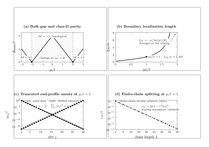
Quantitative diagnostics for the open Kitaev chain with $t=\Delta>0$. Panel (a) shows the bulk gap and class-D parity. Panel (b) shows the amplitude localization length. In panel (c), $L=30$, $\mu/t=1$, $r=-1/2$, and $\xi_M/a=1.443$ is the amplitude length; probability therefore decays with exponent $2/\xi_M$. The plotted end profiles are finite-$L$-normalized, truncated semi-infinite trial Majoranas, not exact finite-chain zero modes, and their far-boundary residual is $\lVert A\boldsymbol v\rVert/t=1.61\times10^{-9}$. In panel (d), dots are high-precision finite-chain secular energies and the dashed curve is the leading large-$L$ asymptote $2t(1-r^2)\lvert r\rvert^L$, not an exact short-chain formula. Original reproducible figure; open the SVG for full-size inspection.

Panel	Quantity shown	Meaning without the graphic
(a)	$E_{\mathrm{gap}}/t=\bigl\lvert\,\lvert\mu/t\rvert-2\,\bigr\rvert$ and $\mathcal M$	The only bulk closings are $\mu/t=\pm2$; $\mathcal M=-1$ between them.
(b)	$\xi_M/a=-1/\ln\lvert\mu/(2t)\rvert$	The amplitude length vanishes at the exactly localized point and diverges on approaching either transition.
(c)	$\lvert\alpha_j\rvert^2$ and the right-end weight	At $L=30$ and $r=-1/2$, the plotted weights are normalized and decay from opposite ends; the underlying signed amplitudes alternate, and the truncated profiles leave only an exponentially small far-boundary residual.
(d)	Exact $E_{\min}/t$ versus $L$ and $2(1-r^2)\lvert r\rvert^L$	The exact secular energy approaches the leading asymptote exponentially; ordinary double-precision diagonalization eventually loses relative accuracy.

Download the reproducible data for the bulk gap and invariant, localization length, normalized end profiles, and finite-chain splitting.

What bulk–boundary correspondence requires

The slogan “nontrivial bulk implies a boundary Majorana” hides hypotheses that determine whether the conclusion is valid.

Ultraviolet completion. A lattice model has a compact Brillouin zone and fixes the Hamiltonian at every momentum. A low-energy continuum expansion near one closing does not, by itself, define a global invariant: a lattice regulator or specified large-momentum completion must say how the mass behaves away from the expansion point.

A specified termination. The invariant predicts modes at an interface between distinct phases, not at an abstract edge. For the open Kitaev chain, the missing bond supplies a definite termination and the vacuum is topologically trivial. Boundary reconstruction may add accidental pairs of low-energy states, but it cannot remove an unpaired class-D Majorana unless the protecting bulk or mobility gap closes, the system leaves the parity-preserving superconducting phase, or the mode couples to another Majorana.

A spectral or mobility gap. Translation symmetry is unnecessary. With disorder, a real-space or scattering invariant can remain quantized while zero-energy bulk states are localized; what must be absent are extended zero-energy channels that destroy the mobility gap. In one-dimensional class D, the zero-energy reflection invariant $Q=\operatorname{sgn}\det r(0)$ changes only at a delocalization transition. Akhmerov et al. 2011, Eqs. (1)–(4) derive this disordered-wire formulation. Rare localized subgap states can nevertheless crowd the spectrum and weaken spectroscopy or braiding gaps.

The correct interacting classification. The BDI integer is a free-fermion result. Symmetry-preserving local interactions can gap eight boundary Majoranas without bilinear symmetry breaking, reducing $\mathbb Z$ to $\mathbb Z_8$; the one-dimensional class-D parity remains $\mathbb Z_2$. Fidkowski and Kitaev 2010, §§ II.A–II.B give the explicit eight-Majorana interaction, and Fidkowski and Kitaev 2011, §§ I–IV develop the interacting classification. In a strongly interacting system, the relevant assumptions concern the many-body gap, fermion parity, and adiabatic equivalence—not merely a single-particle BdG spectrum.

Parity and charging energy. Two Majoranas form one nonlocal fermion, but a floating superconducting island with fixed total parity does not obtain a freely usable two-level system from that pair alone. A charging energy can stabilize charge sectors and enable parity-to-charge protocols. Quasiparticle poisoning changes fermion parity; residual Majorana overlap instead splits the parity sectors, while ordinary Cooper-pair Josephson coupling preserves fermion parity but can compromise charge isolation or mix the intended circuit manifold. The sign relating $i\gamma_1\gamma_2$ to island parity depends on the Majorana-label convention; the physical parity eigenvalue does not. Fu 2010, Eqs. (2)–(4) gives the parity–charge constraint in a mesoscopic topological superconductor.

Chiral p-wave edges and vortices in two dimensions

A regularized continuum representative of a spinless chiral superconductor, with $m>0$ and $\Delta\ne0$, is

$$\mathcal H(\boldsymbol k) =\left(\frac{k^2}{2m}-\mu\right)\tau_z +\Delta k_x\tau_x-\Delta k_y\tau_y.$$

The $k^2\tau_z$ term fixes the direction of the BdG vector at large momentum, allowing the momentum plane to be compactified. The Chern number is computed from the Berry curvature $\Omega_-(\boldsymbol k)$ of the negative-energy BdG band,

$$C=\frac{1}{2\pi}\int d^2k\,\Omega_-(\boldsymbol k).$$

Its sign depends on chirality and orientation, but

$$\mu>0:\ \lvert C\rvert=1, \qquad \mu<0:\ C=0.$$

An interface with $\Delta C\ne0$ has net chirality $\Delta C$ and, after removable counterpropagating pairs are discarded, $\lvert\Delta C\rvert$ protected chiral Majorana branches. The weak-pairing and strong-pairing phases, including their edge and vortex solutions, are developed in Read and Green 2000, §§ II.A–II.B.

For a class-D vortex of integer winding $m$, only the parity of core Majoranas is topologically protected:

$$N_{\mathrm{MZM}}\equiv C\,m\pmod 2.$$

Thus a singly quantized vortex in an odd-Chern phase binds an unpaired Majorana, whereas even $Cm$ permits all core Majoranas to split in symmetry-allowed pairs. This parity is a defect invariant; it does not determine the nonzero Caroli–de Gennes–Matricon spectrum or guarantee a large core minigap. Teo and Kane 2010, § IV.B.3, Eq. (65) place the result in the general classification of topological defects.

Separated vortex zero modes provide the model-level algebra needed for non-Abelian exchange. Ivanov 2001, pp. 268–271 derives the vortex-exchange action. A non-Abelian experimental claim additionally requires controlled motion, conserved parity, splittings small on the protocol timescale, a gap large enough for adiabatic isolation, and a readout that distinguishes the predicted fusion space from ordinary subgap states. Alicea 2012, § 6, pp. 30–31 reviews the wire-network implementation and the operational distinction between possessing zero modes and braiding them.

The semiconductor-wire criterion is a full-gap statement

For the ideal clean, single-subband continuum wire, one common basis gives

$$\mathcal H_{\mathrm{wire}}(k) =\xi_k\tau_z+\alpha k\,\sigma_y\tau_z +V_Z\sigma_x+\Delta_{\mathrm{ind}}\tau_x, \qquad \xi_k=\frac{k^2}{2m^\ast}-\mu.$$

Its positive branches satisfy

$$\begin{aligned} E_\pm^2(k)={}& \xi_k^2+\alpha^2k^2+V_Z^2+\Delta_{\mathrm{ind}}^2\\ &\pm2\sqrt{ V_Z^2(\xi_k^2+\Delta_{\mathrm{ind}}^2) +\alpha^2k^2\xi_k^2 }. \end{aligned}$$

At $k=0$,

$$E_-(0) =\left| \lvert V_Z\rvert-\sqrt{\mu^2+\Delta_{\mathrm{ind}}^2} \right|.$$

The equality $\lvert V_Z\rvert=\sqrt{\mu^2+\Delta_{\mathrm{ind}}^2}$ is the bulk transition, not the topological operating condition. The ideal topological side requires the strict inequality

$$\boxed{\lvert V_Z\rvert>\sqrt{\mu^2+\Delta_{\mathrm{ind}}^2}}$$

and a nonzero full gap,

$$\min_k E_-(k)>0.$$

The second condition is indispensable. For example, if $\alpha=0$, crossings at finite momentum generally make the putative high-field side gapless even though the $k=0$ inequality holds. Finite spin–orbit coupling opens the helical gap, but the usable topological gap can still be much smaller than $\Delta_{\mathrm{ind}}$. Oreg, Refael, and von Oppen 2010, Eqs. (1)–(3) and Lutchyn, Sau, and Das Sarma 2010, Eqs. (1)–(4) and the discussion following Eq. (4) derive the ideal transition and effective spinless regime.

Real devices add occupied subbands, orbital magnetic coupling, field-dependent parent-superconductor suppression, spatially varying electrostatics, interactions, disorder, and contacts. Each can close the minimum gap or generate trivial near-zero Andreev states. Smooth confinement is an explicit trivial mechanism Kells, Meidan, and Brouwer 2012, pp. 100503-1–100503-5, while disorder changes the end-state energy and protection statistics even within the topological regime Brouwer et al. 2011, pp. 196804-1–196804-4. Consequently, satisfying a fitted $k=0$ inequality is neither a measurement of the class-D invariant nor evidence of non-Abelian statistics.

The strongest justified claim

The conclusion must stop at the strongest level supported by the hypotheses and evidence:

1. Model theorem: a specified gapped Hamiltonian has a computed invariant and, for a specified interface or defect, protected boundary-mode parity.
2. Platform identification: an effective Hamiltonian and its full gap describe a material or device over the relevant energy and length scales.
3. Zero-mode identification: nonlocality, stability, and parity response exclude plausible trivial subgap mechanisms.
4. Non-Abelian operation: controlled fusion or exchange acts on the predicted degenerate state space with the required coherence and error bounds.

No earlier level proves a later one. The validity map makes those dependencies and failure points explicit.

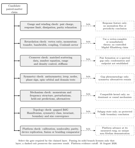
Bulk topology licenses protected modes for a specified model and interface. Device calibration, nonlocal spectroscopy, parity control, and adversarial trivial models are additional obligations. Original schematic, not to scale.

The paired-matter claim test matrix organizes the checks at each level. Current platform-specific evidence belongs on the separate Majorana evidence page.

Common pitfalls

Counting both Nambu partners. The $\pm E$ eigenvectors are redundant partners, not two independent quasiparticles. Keep the $1/2$ in the full-zone Nambu Hamiltonian and compute the two-dimensional Chern number for one energy subspace, conventionally the negative-energy band.

Calling a small eigenvalue a protected zero mode. A short wire, a smooth confinement potential, or an accidental Andreev level can produce a small energy. Verify the bulk invariant, symmetry-preserving stability, spatial profile, length scaling, and boundary or defect hypotheses independently.

Using the transition equality as the topological criterion. At equality the bulk gap is closed and the invariant is undefined. The desired side uses a strict inequality and still requires a positive minimum gap over all momentum.

Confusing amplitude and probability lengths. If the wavefunction amplitude decays as $e^{-x/\xi_M}$, its probability decays as $e^{-2x/\xi_M}$. Quoting a localization length without stating which convention is used creates a factor-of-two ambiguity.

Treating the free BDI integer as interaction-proof. Exact chiral symmetry gives a free-fermion integer, but generic class-D perturbations retain only its parity and symmetry-preserving interactions identify BDI phases modulo eight.

Exercises

1. Particle–hole symmetry and the phase boundaries

Verify $\tau_x\mathcal H(k)^\ast\tau_x=-\mathcal H(-k)$, derive the spectrum, and locate every gap closing for $\Delta\ne0$. Then evaluate $\mathcal M$ in the three intervals separated by the closings.

Solution

$d_z(k)$ is real and even, while $d_y(k)$ is real and odd. Complex conjugation changes $\tau_y\to-\tau_y$; conjugation by $\tau_x$ changes both $\tau_z$ and $\tau_y$ in sign. Hence $\tau_x\mathcal H(k)^\ast\tau_x=-d_z(k)\tau_z+d_y(k)\tau_y=-\mathcal H(-k)$.

Because $\tau_y$ and $\tau_z$ anticommute and square to one,

$$E_\pm^2(k)=d_z^2(k)+d_y^2(k) =(\mu+2t\cos k)^2+4\Delta^2\sin^2k.$$

For $\Delta\ne0$, $d_y=0$ only at $k=0,\pi$. At $k=0$, $d_z=0$ gives $\mu=-2t$; at $k=\pi$, it gives $\mu=2t$. For $t>0$,

$$\mathcal M= \begin{cases} +1, & \mu<-2t,\\ -1, & -2t<\mu<2t,\\ +1, & \mu>2t. \end{cases}$$

At the two endpoints the spectrum is gapless and $\mathcal M$ is not defined.

2. Normalize the end mode and measure its finite-chain error

At $t=\Delta>0$ and $\lvert r\rvert<1$, normalize $\Gamma_L=\sum_{j=1}^L\alpha_j a_j$ with $\alpha_j\propto r^{j-1}$. Construct the unit-norm Nambu vector and compute the residual caused by the right boundary.

Solution

The Majorana convention $\Gamma_L^2=1$ requires $\sum_j\alpha_j^2=1$. The geometric sum gives

$$\alpha_j=\mathcal N_Lr^{j-1}, \qquad \mathcal N_L=\sqrt{\frac{1-r^2}{1-r^{2L}}}.$$

The Nambu vector is $\Phi_L=2^{-1/2}(\boldsymbol\alpha,\boldsymbol\alpha)^T$, so $\Phi_L^\dagger\Phi_L=1$ and $\mathcal C\Phi_L=\Phi_L$. The recurrence $2t\alpha_{j+1}+\mu\alpha_j=0$ holds through $j=L-1$. At the last site there is no $\alpha_{L+1}$, leaving

$$\lVert A\boldsymbol v_L\rVert =\lvert\mu\alpha_L\rvert =2t\,\mathcal N_L\lvert r\rvert^L.$$

Thus finite-$L$ normalization does not turn the truncated semi-infinite profile into an exact finite-chain zero eigenvector.

3. Read the localization and splitting diagnostics

Set $\mu/t=1$, $t=\Delta>0$. Find $r$, $\xi_M/a$, the probability decay exponent, and the leading $E_{\min}/t$ at $L=10$ and $L=30$. Compare the $L=10$ estimate with the exact secular data.

Solution

Here $r=-1/2$, so

$$\frac{\xi_M}{a}=\frac{1}{\ln2}=1.442695\ldots, \qquad \lvert\alpha_j\rvert^2\propto e^{-2(j-1)a/\xi_M}.$$

The leading splitting is

$$\frac{E_{\min}}{t}\sim 2(1-r^2)\lvert r\rvert^L =\frac32\,2^{-L}.$$

Therefore

$$\frac{E_{\min}(10)}{t}\sim1.46484375\times10^{-3}, \qquad \frac{E_{\min}(30)}{t}\sim1.39698386\times10^{-9}.$$

The high-precision splitting data give $E_{\min}(10)/t=1.46485387831\times10^{-3}$, a relative asymptotic error of about $6.9\times10^{-6}$. By $L=30$, the exact value agrees with the displayed asymptote to the quoted digits.

4. Apply parity tests without overclaiming

(a) State the protected vortex-Majorana parity for $(C,m)=(1,1)$, $(2,1)$, and $(1,2)$.

(b) An ideal single-subband wire has $\mu=0.60\,\mathrm{meV}$ and $\Delta_{\mathrm{ind}}=0.25\,\mathrm{meV}$. Find the critical $\lvert V_Z\rvert$ and state what must still be checked above it.

Solution

(a) Since $N_{\mathrm{MZM}}\equiv Cm\pmod2$, the three parities are odd, even, and even. Only the first case forces an unpaired class-D vortex Majorana. “Even” does not forbid low-energy core states; it means topology permits them to split in pairs.

(b)

$$\lvert V_Z\rvert_c =\sqrt{(0.60\,\mathrm{meV})^2+(0.25\,\mathrm{meV})^2} =0.65\,\mathrm{meV}.$$

The ideal topological side requires $\lvert V_Z\rvert>0.65\,\mathrm{meV}$, not equality. One must also verify $\min_kE_-(k)>0$, finite spin–orbit coupling, the occupied-subband structure, survival of the parent and induced gaps, and the effects of orbital coupling, electrostatic inhomogeneity, interactions, disorder, and contacts. Even those checks establish an effective topological phase, not non-Abelian operation.

References

• Akhmerov, A. R., Dahlhaus, J. P., Hassler, F., Wimmer, M., and Beenakker, C. W. J. (2011). “Quantized conductance at the Majorana phase transition in a disordered superconducting wire.” Physical Review Letters 106, 057001. doi:10.1103/PhysRevLett.106.057001.
• Alicea, J. (2012). “New directions in the pursuit of Majorana fermions in solid state systems.” Reports on Progress in Physics 75(7), 076501. doi:10.1088/0034-4885/75/7/076501.
• Brouwer, P. W., Duckheim, M., Romito, A., and von Oppen, F. (2011). “Probability distribution of Majorana end-state energies in disordered wires.” Physical Review Letters 107, 196804. doi:10.1103/PhysRevLett.107.196804.
• Fidkowski, L., and Kitaev, A. (2010). “Effects of interactions on the topological classification of free fermion systems.” Physical Review B 81, 134509. doi:10.1103/PhysRevB.81.134509.
• Fidkowski, L., and Kitaev, A. (2011). “Topological phases of fermions in one dimension.” Physical Review B 83, 075103. doi:10.1103/PhysRevB.83.075103.
• Fu, L. (2010). “Electron teleportation via Majorana bound states in a mesoscopic superconductor.” Physical Review Letters 104, 056402. doi:10.1103/PhysRevLett.104.056402.
• Ivanov, D. A. (2001). “Non-Abelian statistics of half-quantum vortices in $p$-wave superconductors.” Physical Review Letters 86, 268–271. doi:10.1103/PhysRevLett.86.268.
• Kells, G., Meidan, D., and Brouwer, P. W. (2012). “Near-zero-energy end states in topologically trivial spin-orbit coupled superconducting nanowires with a smooth confinement.” Physical Review B 86, 100503(R). doi:10.1103/PhysRevB.86.100503.
• Kitaev, A. Yu. (2001). “Unpaired Majorana fermions in quantum wires.” Physics-Uspekhi 44(10S), 131–136. doi:10.1070/1063-7869/44/10S/S29.
• Lutchyn, R. M., Sau, J. D., and Das Sarma, S. (2010). “Majorana fermions and a topological phase transition in semiconductor–superconductor heterostructures.” Physical Review Letters 105, 077001. doi:10.1103/PhysRevLett.105.077001.
• Oreg, Y., Refael, G., and von Oppen, F. (2010). “Helical liquids and Majorana bound states in quantum wires.” Physical Review Letters 105, 177002. doi:10.1103/PhysRevLett.105.177002.
• Read, N., and Green, D. (2000). “Paired states of fermions in two dimensions with breaking of parity and time-reversal symmetries and the fractional quantum Hall effect.” Physical Review B 61, 10267–10297. doi:10.1103/PhysRevB.61.10267.
• Teo, J. C. Y., and Kane, C. L. (2010). “Topological defects and gapless modes in insulators and superconductors.” Physical Review B 82, 115120. doi:10.1103/PhysRevB.82.115120.