The Fermi Gas and Fermi-Surface Kinematics

At zero temperature, a uniform noninteracting Fermi gas fills every one-particle state with energy below the chemical potential. For an isotropic quadratic dispersion, the occupied momenta form a ball—the Fermi sea—whose boundary is the Fermi surface. Removing a fermion just inside this boundary or adding one just outside it costs arbitrarily little energy. Low-energy physics is therefore organized by a thin shell around a codimension-one surface, not by momenta near a single point.

This page works in $d$ spatial dimensions with $\hbar=k_{\mathrm B}=1$, volume $V$, quadratic dispersion $\epsilon_{\mathbf k}=k^2/(2m)$, and a declared spin or flavor degeneracy $g$. The free spherical gas is the model; anisotropic bands, interacting volume theorems, and quasiparticle dynamics enter only after the kinematics is secure.

Required background. Second-quantized fermions supplies the occupation-number algebra and continuum normalization. Finite-density ensembles supplies the role of $H-\mu N$ and the zero-temperature Fermi–Dirac limit. Helpful background. Fourier and Plancherel conventions explain the replacement of a box momentum sum by an integral.

The filled sea and its boundary

In a periodic box, the grand-canonical free Hamiltonian is

$$H-\mu N =\sum_{\mathbf k,a} \bigl(\epsilon_{\mathbf k}-\mu\bigr) c_{\mathbf k a}^{\dagger}c_{\mathbf k a}, \qquad a=1,\ldots,g.$$

Each mode can be occupied at most once for each value of $a$. At $T=0$, minimizing $H-\mu N$ therefore gives

$$n_{\mathbf k a} =\Theta\!\left(\mu-\epsilon_{\mathbf k}\right).$$

For the quadratic dispersion, $\mu=E_F=k_F^2/(2m)$ and the occupied region is $k<k_F$. Its boundary $k=k_F$ is the Fermi surface. The terminology matters: the sea is a $d$-dimensional region of occupied states, whereas its surface has dimension $d-1$. In one dimension the “surface” consists of the two points $-k_F$ and $+k_F$.

The number density follows directly from one state per momentum-space cell $(2\pi)^d/V$ and per internal label:

$$\begin{aligned} n &=g\int_{k<k_F}\frac{\mathrm d^d k}{(2\pi)^d}\\ &=\frac{gS_{d-1}}{d(2\pi)^d}k_F^d, \qquad S_{d-1}=\frac{2\pi^{d/2}}{\Gamma(d/2)}. \end{aligned}$$

This equation translates density into a momentum scale. The common cases are worth keeping side by side:

Spatial dimension	Occupied region	Density $n$	Density of states at $E_F$
$d=1$	interval $[-k_F,k_F]$	$gk_F/\pi$	$gm/(\pi k_F)$
$d=2$	disk	$gk_F^2/(4\pi)$	$gm/(2\pi)$
$d=3$	ball	$gk_F^3/(6\pi^2)$	$gmk_F/(2\pi^2)$

Every entry includes all $g$ internal species. A source quoting a per-spin density of states differs by a factor of $g$ even though the physical system has not changed. The state count and its three-dimensional specialization are derived pedagogically in Tong 2012, §§ 3.1 and 3.6.1–3.6.2.

Density of states and thermodynamic checks

Let $\nu(\epsilon)$ denote the number of one-particle states per unit volume, per unit energy, including the declared degeneracy $g$:

$$\nu(\epsilon) =g\int\frac{\mathrm d^d k}{(2\pi)^d} \delta\!\left(\epsilon-\epsilon_{\mathbf k}\right).$$

The delta function converts a radial energy interval into momentum shells. For a rotationally invariant dispersion, let $k_i>0$ run over the simple roots of $\epsilon(k_i)=\epsilon$. Then

$$\nu(\epsilon) =\frac{gS_{d-1}}{(2\pi)^d} \sum_i \frac{k_i^{d-1}}{\lvert\epsilon'(k_i)\rvert}.$$

A monotone radial band has only one such root. For $\epsilon_k=k^2/(2m)$ this gives

$$\nu(\epsilon) =\frac{gS_{d-1}m}{(2\pi)^d} (2m\epsilon)^{(d-2)/2}.$$

Downstream pages use $N(0)\equiv\nu(E_F)$ for this total density of states. The zero in $N(0)$ means zero excitation energy $\xi=\epsilon-E_F$, not zero one-particle energy.

Several independent identities check the normalization. Differentiating the state count gives

$$\frac{\partial n}{\partial E_F}=\nu(E_F).$$

Direct integration of the filled sea gives the ground-state energy density and pressure,

$$\frac{E_0}{V}=\frac{d}{d+2}nE_F, \qquad P=\frac{2}{d}\frac{E_0}{V} =\frac{2}{d+2}nE_F.$$

The first identity checks the Fermi-surface measure; the second is the nonrelativistic virial relation for a free quadratic dispersion. At fixed density, a smooth density of states also gives the leading low-temperature heat capacity

$$\frac{C_V}{V} =\frac{\pi^2}{3}\nu(E_F)T+O(T^3).$$

Only a fraction of order $T/E_F$ of the fermions can be thermally rearranged, because states deep inside the sea are Pauli blocked. This is why the heat capacity is linear in $T$, rather than of order $n$ as in a classical gas. The heuristic and the fixed-density Sommerfeld calculation are developed in Tong 2012, §§ 3.6.3–3.6.4, pp. 95–100.

Linearization around a smooth surface

The spherical gas makes the local geometry explicit. Choose a point $\mathbf k_F=k_F\hat{\mathbf n}$ and decompose a nearby displacement as

$$\mathbf k =\mathbf k_F+k_\perp\hat{\mathbf n}+\mathbf k_\parallel, \qquad \hat{\mathbf n}\mathbin{\cdot}\mathbf k_\parallel=0.$$

Then the excitation energy is

$$\begin{aligned} \xi_{\mathbf k} &\equiv\epsilon_{\mathbf k}-E_F\\ &=v_Fk_\perp +\frac{k_\perp^2+k_\parallel^2}{2m}, \qquad v_F=\frac{k_F}{m}. \end{aligned}$$

To leading order, energy measures displacement normal to the surface. Tangential momentum first enters through curvature. Consequently, the states with $\lvert\xi_{\mathbf k}\rvert<\Lambda_E\ll E_F$ occupy a shell of half-thickness $\Lambda_E/v_F$ on either side of the surface—a total normal thickness $2\Lambda_E/v_F$—while retaining an entire $(d-1)$-dimensional set of tangential labels. Indeed,

$$g\int_{\lvert\xi_{\mathbf k}\rvert<\Lambda_E} \frac{\mathrm d^d k}{(2\pi)^d} =2\nu(E_F)\Lambda_E +\frac{1}{3}\nu''(E_F)\Lambda_E^3 +O(\Lambda_E^5)$$

when $\nu(\epsilon)$ is sufficiently smooth throughout the symmetric energy window. Odd terms in its Taylor series integrate to zero. This codimension-one phase space is the reason a Fermi surface cannot be treated like an isolated relativistic vacuum at $\mathbf k=0$.

For a general differentiable band, the same construction works wherever

$$\mathbf v_F(\mathbf k_F) =\boldsymbol\nabla_{\mathbf k}\epsilon_{\mathbf k}\big|_{\mathbf k_F}$$

is nonzero. The local normal points along $\mathbf v_F$, and the density of states is the surface integral

$$\nu(E_F) =\frac{g}{(2\pi)^d} \int_{\mathrm{FS}} \frac{\mathrm dS_{\mathbf k}}{\lvert\mathbf v_F(\mathbf k)\rvert}.$$

This formula explains both the abundance of low-energy states and the danger of a van Hove point: where $\mathbf v_F=0$, the regular-surface approximation fails and the density of states can become singular.

The schematic below shows what this local kinematics feeds. Inspect the four branches separately: a Green-function pole, Landau response, a Fermi-volume statement, and an interaction-channel flow are related, but none automatically proves the others.

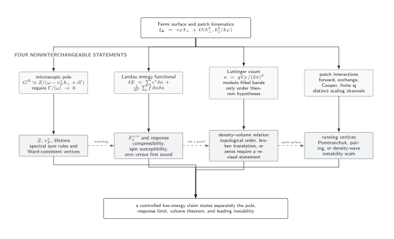
A smooth Fermi surface supplies the common low-energy geometry for four logically distinct claims. The map is schematic and not to scale; its local expansion retains normal motion at first order and tangential curvature at second order. Pole longevity, response limits, volume-theorem hypotheses, and instability control must still be checked independently.

Here $H_{ij}=e_i^ae_j^b\,\partial_{k_a}\partial_{k_b}\epsilon_{\mathbf k}|_{\mathbf k_F}$ is the band Hessian restricted to an orthonormal tangent basis, with repeated tangential indices summed. Also, $Z$ is the pole residue, $\Gamma$ its linewidth, $V_{{\rm occ},a}$ is an occupied continuum volume, $V^{\rm or}_{F,a}$ is an oriented lattice-pocket volume (electron pockets positive and hole pockets negative), $V_{\mathrm{BZ}}$ is the Brillouin-zone volume, and $F_\alpha$ is a generic response-channel eigenvalue. The latter specializes to the familiar $F_\ell^{s,a}$ for an SU(2)-symmetric spin-$1/2$ liquid. Dashed connectors mark matching or shared geometry, not logical implication. On a lattice, $n_{\mathrm{cell}}$ is the dimensionless particle number per physical unit cell, so filled bands contribute integers rather than dimensional densities; see Oshikawa 2000, Eq. (7), pp. 3371–3372. The chapter’s claim-comparison table spells out the hypotheses and failure tests behind every branch.

Particle–hole excitations

A neutral excitation removes an occupied fermion of momentum $\mathbf k$ and creates one at $\mathbf k+\mathbf q$ outside the sea:

$$\lvert\mathbf k;\mathbf q\rangle =c_{\mathbf k+\mathbf q,a}^{\dagger} c_{\mathbf k a}\lvert\mathrm{FS}\rangle.$$

It carries momentum $\mathbf q$ and, for the quadratic gas, energy

$$\omega =\epsilon_{\mathbf k+\mathbf q}-\epsilon_{\mathbf k} =\frac{\mathbf k\mathbin{\cdot}\mathbf q}{m} +\frac{q^2}{2m},$$

subject to $k<k_F$ and $\lvert\mathbf k+\mathbf q\rvert>k_F$. These occupation inequalities are as important as the energy formula.

In $d\ge2$, the original Fermi surface and a copy shifted by $-\mathbf q$ intersect for $q<2k_F$. Initial and final momenta can then lie arbitrarily close to the surface, so the particle–hole continuum reaches arbitrarily small positive energy even when $q$ is not infinitesimal. For the isotropic gas its upper edge is

$$\omega_+(q)=v_Fq+\frac{q^2}{2m},$$

while the lower edge is

$$\omega_-(q)= \begin{cases} 0, & 0<q\le2k_F,\\[2pt] \dfrac{q^2}{2m}-v_Fq, & q>2k_F. \end{cases}$$

The interval between these edges is kinematically available; a response function additionally weights it with matrix elements and occupation factors. In one dimension the two-point “surface” leaves much less angular freedom, so low-energy channels are concentrated near momentum transfer $q\simeq0$ or $q\simeq2k_F$. The Lindhard-function page turns this phase space into a retarded density response.

The coexistence of small excitation energy with a continuum of momenta has several consequences. Forward scattering probes nearby patches, nearly back-to-back momenta form the exceptional Cooper channel, and finite-$q$ geometry can enhance density-wave tendencies when pieces of the surface are nested. The higher-dimensional scaling, forward and Cooper channels, and nesting analysis are developed in Shankar 1994, §§ V–VII and IX–X, pp. 159–185.

Beyond the spherical free gas

The durable object is a regular level set $\epsilon_{n\mathbf k}=\mu$, not necessarily a sphere. Several changes must be made explicitly:

• Several pockets or bands. Sum the occupied momentum-space regions and the surface integrals over every relevant band and pocket, with each degeneracy stated. A “hole volume” is shorthand relative to a completely filled band, so its sign convention must be explicit.
• A lattice. Momentum lives in a Brillouin zone. Completely filled bands and the physical unit cell matter, so continuum counting cannot be copied without translation.
• Finite temperature. The sharp step is rounded over $\lvert\epsilon-\mu(T)\rvert\sim T$. The zero-temperature $E_F$ remains a useful scale when $T\ll E_F$, but $\mu(T)$ need not equal $E_F$ exactly.
• Interactions. A singular surface of the exact Green function may persist, but its volume and its relation to density require the hypotheses of Luttinger’s theorem. A volume count alone does not establish a long-lived quasiparticle pole.
• Singular geometry. Van Hove points, band touchings, perfectly flat directions, and nesting invalidate the generic smooth-surface expansion and can change the low-energy scaling.

These qualifications mark the boundary of the free model rather than defects in it. The free gas supplies the normalization and geometry against which interacting and lattice statements are checked.

Common pitfalls

Confusing the Fermi sea with the Fermi surface. The sea contains all occupied zero-temperature momenta; the surface is only its boundary. Low-energy excitations live near the boundary even though most particles remain deep in the sea.

Leaving spin or flavor implicit. Both $n$ and $\nu(E_F)$ scale with $g$. Translate a per-species density of states to the total convention before comparing heat capacities, susceptibilities, or Landau parameters.

Dropping curvature everywhere. The linear term controls energy normal to a regular patch, but tangential curvature decides whether separated patches intersect, nest, or support a particular momentum transfer. It is subleading locally, not globally irrelevant.

Promoting free counting to an interacting theorem. The free relation between occupied volume and density follows from literal occupation numbers. Its interacting analogue has symmetry, analyticity, unit-cell, and sometimes topological hypotheses.

Exercises

State counting in two dimensions

For a spin-$1/2$ quadratic gas in $d=2$, derive $k_F$ as a function of the total density and show that the total density of states is independent of energy.

Solution

With $g=2$, the occupied disk has area $\pi k_F^2$, so

$$n=2\frac{\pi k_F^2}{(2\pi)^2} =\frac{k_F^2}{2\pi}, \qquad k_F=\sqrt{2\pi n}.$$

Because $k(\epsilon)=\sqrt{2m\epsilon}$ and $v(k)=k/m$,

$$\nu(\epsilon) =2\frac{2\pi}{(2\pi)^2}\frac{k}{k/m} =\frac{m}{\pi}.$$

The $k$ from the circumference cancels the $1/k$ from converting a momentum interval to an energy interval.

Ground-state energy check

Starting from the momentum integral, show in arbitrary $d$ that $E_0/V=dnE_F/(d+2)$.

Solution

Radial integration gives

$$\frac{E_0}{V} =\frac{gS_{d-1}}{(2\pi)^d} \int_0^{k_F}\mathrm dk\,k^{d-1}\frac{k^2}{2m} =\frac{gS_{d-1}}{(2\pi)^d} \frac{k_F^{d+2}}{2m(d+2)}.$$

Using $n=gS_{d-1}k_F^d/[d(2\pi)^d]$ and $E_F=k_F^2/(2m)$ yields $E_0/V=dnE_F/(d+2)$.

Patch expansion and shell count

For the spherical quadratic gas, derive the expansion of $\xi_{\mathbf k}$ around $\mathbf k_F=k_F\hat{\mathbf n}$. Then Taylor-expand the density of states to show why the symmetric shell count has no term proportional to $\Lambda_E^2$.

Solution

Write $\mathbf k=\mathbf k_F+k_\perp\hat{\mathbf n}+\mathbf k_\parallel$ with $\hat{\mathbf n}\mathbin{\cdot}\mathbf k_\parallel=0$. Subtracting $E_F=k_F^2/(2m)$ gives

$$\xi_{\mathbf k} =\frac{2k_Fk_\perp+k_\perp^2+k_\parallel^2}{2m} =v_Fk_\perp+\frac{k_\perp^2+k_\parallel^2}{2m}.$$

For the shell count, put $x=\epsilon-E_F$ and expand

$$\nu(E_F+x) =\nu(E_F)+\nu'(E_F)x +\frac{1}{2}\nu''(E_F)x^2 +\frac{1}{6}\nu'''(E_F)x^3+O(x^4).$$

Integrating from $-\Lambda_E$ to $+\Lambda_E$ cancels every odd term, so

$$\int_{-\Lambda_E}^{\Lambda_E}\!\mathrm dx\,\nu(E_F+x) =2\nu(E_F)\Lambda_E +\frac{1}{3}\nu''(E_F)\Lambda_E^3 +O(\Lambda_E^5).$$

The leading factor of two counts the inner and outer half-shells.

Threshold of the particle–hole continuum

For $d\ge2$, explain geometrically why the lower edge is zero for $q<2k_F$, and derive the positive lower edge for $q>2k_F$.

Solution

For $q<2k_F$, two spheres of radius $k_F$ whose centers are separated by $q$ intersect. One may choose $\mathbf k$ just inside the original surface and $\mathbf k+\mathbf q$ just outside it near an intersection, making $\omega$ arbitrarily small and positive.

For $q>2k_F$, the surfaces do not intersect. The infimum occurs as $\mathbf k$ approaches the Fermi surface from inside, opposite to $\mathbf q$, so $\mathbf k\mathbin{\cdot}\mathbf q\to-k_Fq$. Therefore

$$\omega_-(q) =\frac{q^2}{2m}-\frac{k_Fq}{m} =\frac{q^2}{2m}-v_Fq>0.$$

Continue

Landau Fermi-liquid theory replaces the free occupation energy by a quasiparticle energy functional. Microscopic quasiparticle criteria determine when an interacting Green function actually has a long-lived pole. Fermi-surface patch theory turns the normal-shell geometry into low-energy power counting. The chapter’s claim-comparison table keeps those statements separate from Luttinger counting and instability evidence.

References

• Oshikawa, Masaki. “Topological Approach to Luttinger’s Theorem and the Fermi Surface of a Kondo Lattice.” Physical Review Letters 84 (2000): 3370–3373. DOI.
• Shankar, Ramamurti. “Renormalization-Group Approach to Interacting Fermions.” Reviews of Modern Physics 66 (1994): 129–192. §§ V–VII and IX–X. DOI.
• Tong, David. Lectures on Statistical Physics. Cambridge: University of Cambridge, 2012. §§ 3.1 and 3.6. Course notes.

Further reading

• Fetter, Alexander L., and John Dirk Walecka. Quantum Theory of Many-Particle Systems. New York: McGraw–Hill, 1971; reprint, Mineola, NY: Dover, 2003. Publisher record.