The Anderson Impurity Model and Hybridization

The single-impurity Anderson model is the minimal quantum theory in which a localized orbital can fluctuate among empty, singly occupied, and doubly occupied states while repelling a second electron. Its three basic inputs—level position $\varepsilon_d$, repulsion $U$, and hybridization function $\Delta$—separate empty-orbital, mixed-valence, and local-moment behavior. The model is also the charge-fluctuating parent of the Kondo model, but that reduction is controlled only when both charge excitations are well separated from the low-energy window.

This page first solves the noninteracting resonant level exactly, because its causality, width, and sum rule are indispensable checks on every interacting solver. It then restores $U$, identifies the atomic charge gaps, and explains why a local-moment regime in a metal must not be mistaken for static symmetry breaking or for the eventual screened ground state.

Required background. Impurity models and local moments supplies the bath, channel, and scale definitions.

Helpful background. Dyson equations supplies the hybridization self-energy. Lehmann representations supplies positivity and spectral normalization.

Charge sectors of the Anderson orbital

With the chemical potential absorbed into all one-particle energies, the spin-degenerate model is

$$\begin{aligned} H={}&\sum_{k\sigma}\varepsilon_k c_{k\sigma}^\dagger c_{k\sigma} +\varepsilon_d\sum_\sigma n_{d\sigma} +U n_{d\uparrow}n_{d\downarrow}\\ &+\sum_{k\sigma} \left(V_kc_{k\sigma}^\dagger d_\sigma +V_k^\ast d_\sigma^\dagger c_{k\sigma}\right). \end{aligned}$$

For $V_k=0$, the four local states and their energies are

Local state	Charge	Spin	Energy
$\lvert0\rangle$	0	0	$E_0=0$
$\lvert\uparrow\rangle,\lvert\downarrow\rangle$	1	$1/2$	$E_1=\varepsilon_d$
$\lvert\uparrow\downarrow\rangle$	2	0	$E_2=2\varepsilon_d+U$

For repulsive $U>0$, single occupancy is the atomic ground sector when

$$-U<\varepsilon_d<0.$$

Measured from that sector, the removal and addition gaps are

$$E_-=-\varepsilon_d, \qquad E_+=\varepsilon_d+U.$$

The empty and singly occupied sectors become degenerate at $\varepsilon_d=0$; the singly and doubly occupied sectors become degenerate at $\varepsilon_d=-U$. For an ordinary metallic bath with $\Gamma(0)>0$, hybridization rounds these atomic boundaries into charge-fluctuation crossovers. A pseudogap or hard-gap bath can instead retain a level crossing or support an impurity quantum phase transition, so that qualification matters. A useful first classification for the metallic case is therefore

Regime	Atomic location	Hybridized diagnostic
Empty orbital	$\varepsilon_d$ well above the Fermi level	$\langle n_d\rangle\ll1$ and no separated spin doublet
Local moment	$E_-,E_+\gg\Gamma_\ast,T$	$\langle n_d\rangle\simeq1$, small charge response, and an intermediate Curie window
Mixed valence	either charge gap is comparable to broadening or temperature	adjacent charge sectors both have appreciable probability
Doubly occupied	$\varepsilon_d+U$ well below the Fermi level	$\langle n_d\rangle\simeq2$ and no separated spin doublet

The inequalities identify scale regimes, not phase boundaries of the ordinary metallic single-impurity model. Anderson’s original paper introduced the Hamiltonian and analyzed moment formation in unrestricted Hartree–Fock theory; the exact quantum model does not acquire a static spin expectation value at a finite, symmetry-preserving impurity. Anderson 1961, §§II–IV, pp. 42–46 should be read with that approximation explicit. Hewson 1993, ch. 1 develops the model, its charge regimes, and the Anderson-to-Kondo limit beyond that historical mean-field framing.

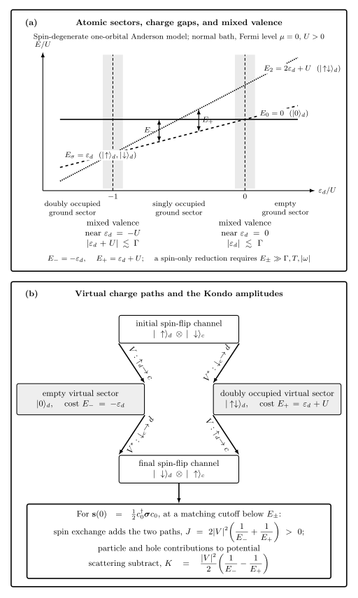
The upper panel of the next figure displays the atomic energies and the two positive gaps in the local-moment window. The lower panel anticipates how those same gaps enter the controlled charge-elimination step on the next page.

On a narrow screen, swipe the diagram or focus it and use the left/right arrow keys; Home and End move to its edges. Open the full-size diagram.

Anderson charge sectors and their low-energy virtual paths. In the local-moment window, removing the impurity electron costs $E_-=-\varepsilon_d$ and adding the opposite spin costs $E_+=\varepsilon_d+U$. Both paths return to charge one and later add in the antiferromagnetic exchange, while their spin-independent potential-scattering contributions have opposite signs. Original schematic at a Fermi level set to zero; not to scale.

The exact resonant-level checkpoint

Set $U=0$. The equations of motion can then be solved without approximation. Eliminating the bath amplitudes gives

$$G_{d,0}^R(\omega) =\frac{1} {\omega+i0^+-\varepsilon_d-\Delta^R(\omega)},$$

where

$$\Delta^R(\omega) =\sum_k\frac{\lvert V_k\rvert^2} {\omega-\varepsilon_k+i0^+} =\Lambda(\omega)-i\Gamma(\omega).$$

The sign is fixed by retarded causality: $\Gamma(\omega)\ge0$ and $\operatorname{Im}\Delta^R\le0$. In the volume convention

$$A_d(\omega)=-2\operatorname{Im}G_d^R(\omega),$$

it is convenient on this page to use the unit-normalized density $\mathcal A_d=A_d/(2\pi)$. The continuum part of the exact noninteracting result is

$$\mathcal A_{d,0}(\omega) =\frac{1}{\pi} \frac{\Gamma(\omega)} {[\omega-\varepsilon_d-\Lambda(\omega)]^2 +\Gamma^2(\omega)}.$$

For a physical finite-band model it obeys

$$\int_{-\infty}^{\infty}\!\mathrm d\omega\, \mathcal A_{d,0}(\omega)=1$$

per spin, including any bound-state delta functions outside the continuum that are not displayed in the preceding continuum formula. This normalization follows from $G_{d,0}(z)\sim1/z$ at large $z$ and is a stricter test than merely obtaining a positive-looking peak.

In the wide, flat-band limit, absorb the slowly varying $\Lambda$ into a renormalized $\varepsilon_d$ and put $\Gamma(\omega)\simeq\Gamma$. Then

$$\mathcal A_{d,0}(\omega) =\frac{1}{\pi} \frac{\Gamma}{(\omega-\varepsilon_d)^2+\Gamma^2}.$$

The spectral full width at half maximum is $2\Gamma$, while the retarded amplitude decays as $e^{-\Gamma t}$. Confusing those two conventions creates a factor-of-two lifetime error. At zero temperature the occupancy is also analytic:

$$n_{d\sigma} =\int_{-\infty}^{0}\!\mathrm d\omega\, \mathcal A_{d,0}(\omega) =\frac12-\frac1\pi \arctan\!\left(\frac{\varepsilon_d}{\Gamma}\right).$$

This smooth step is the simplest picture of mixed valence: when a level lies within roughly one width of the Fermi energy, empty and occupied configurations are both active. Bulla, Costi, and Pruschke 2008, §II.A, pp. 399–402 uses the same hybridization function as the complete bath input to the numerical impurity problem.

Interactions, spectral weight, and particle–hole symmetry

Restoring $U$ does not change the canonical sum rule, but it redistributes the weight. In the atomic limit, the exact spectral density for spin $\sigma$ is

$$\mathcal A_{d\sigma}^{\mathrm{at}}(\omega) =\bigl(1-\langle n_{d\bar\sigma}\rangle\bigr) \delta(\omega-\varepsilon_d) +\langle n_{d\bar\sigma}\rangle \delta(\omega-\varepsilon_d-U).$$

The first transition adds a $\sigma$ electron when the opposite spin is absent; the second pays $U$ because the opposite spin is present. Hybridization broadens and shifts these charge-transfer features. In a metallic, screened local-moment regime, many-body spin fluctuations also produce a narrow low-energy resonance on the Kondo scale.

The familiar “two Hubbard peaks plus one Kondo peak” is therefore a useful limiting picture, not a universal decomposition into three independent levels. Peaks can overlap in mixed valence, disappear into a band edge, split in a field, or become asymmetric in a structured bath. Their integrated weights must still add to one per spin, and a low-energy peak is not by itself proof of Kondo screening.

For a particle–hole-symmetric bath, the full Hamiltonian is particle–hole symmetric at

$$\varepsilon_d=-\frac U2.$$

Then $E_-=E_+=U/2$, $\langle n_d\rangle=1$, and the local spectrum is symmetric about the Fermi energy. On the next page, the two charge paths give equal exchange contributions while potential scattering cancels. Detuning from this point does not destroy the local moment immediately; it makes empty and doubly occupied virtual fluctuations unequal.

The local-moment requirement is stronger than the atomic inequality $-U<\varepsilon_d<0$. In particular, the charge susceptibility $\chi_c=-\partial\langle n_d\rangle/\partial\varepsilon_d$ should be small compared with its mixed-valence value, and

$$\frac{\Gamma_\ast}{E_-}\ll1, \qquad \frac{\Gamma_\ast}{E_+}\ll1.$$

These ratios control a spin-only reduction. When either is order one, a Kondo Hamiltonian throws away an active charge state and its apparent Kondo scale is not a controlled prediction.

Where the wide-band model stops

The constant-$\Gamma$ approximation is reliable only when both $\Gamma(\omega)$ and its Hilbert-transform partner $\Lambda(\omega)$ vary slowly across every scale used in the calculation. It fails near a band edge, van Hove singularity, pseudogap, superconducting gap, narrow lead resonance, or molecular interference zero. A real solution of

$$\omega-\varepsilon_d-\Lambda(\omega)=0$$

outside the continuum can create a bound-state delta function that a Lorentzian fit entirely misses.

Multiple orbitals require matrix-valued one-particle energies and hybridization $\Delta$, together with an interaction tensor containing intra- and interorbital repulsion, Hund exchange, and pair hopping. Crystal fields and Hund coupling can select a different local multiplet, while off-diagonal hybridization can rotate the active orbital basis with frequency. A quantum dot inherits still more calibration: charging energies, level spacing, lead modes, capacitive voltage division, and nonequilibrium occupation. The one-orbital model is powerful precisely because each of these omissions can be named and tested.

The chapter map places this one-orbital Anderson model between bath specification and charge elimination. Its hybridization has one active eigenchannel, so this route supplies the $k=1$ Kondo theory; genuine $k>1$ screening follows the separate channel-preserving input and matching lane. The map is shown again here as an orientation aid; the detailed charge-state figure above is the page-specific diagnostic.

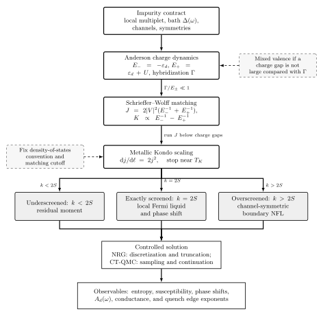
The Anderson model retains real and virtual charge fluctuations. Only the branch with both charge gaps large compared with hybridization and external scales licenses the displayed spin-only matching step, and this one-orbital route has $k=1$. The separate multichannel lane requires a microscopic realization with equivalent conserved baths and channel-resolved exchanges before the $k$ versus $2S$ classification applies. Original schematic, not to scale.

The impurity claim test matrix pairs each regime with a sum-rule, causality, or charge-fluctuation failure test.

When both charge-control ratios are small, continue to Anderson-to-Kondo matching; otherwise retain the charge-fluctuating Anderson model.

Common pitfalls

Calling the Hartree–Fock saddle a permanent impurity magnet. A symmetry-broken mean-field solution can diagnose a tendency to moment formation, but the exact metallic single impurity undergoes Kondo screening at sufficiently low energy when its hypotheses hold. State the temperature window and observable.

Dropping the real hybridization shift. A constant $\Lambda$ may be absorbed into $\varepsilon_d$, but a frequency-dependent shift changes peak positions and can create bound states. Causality ties it to $\Gamma$.

Calling every zero-energy resonance “Kondo.” The $U=0$ resonant level already produces a Lorentzian at the Fermi energy when $\varepsilon_d=0$. Kondo identification additionally requires a separated moment regime and the correct temperature, field, entropy, or scaling behavior.

Exercises

1. Derive the resonant-level propagator. Starting from the $U=0$ equations of motion for $G_{dd}^R$ and $G_{kd}^R$, eliminate the bath Green functions and recover $G_{d,0}^R$.

Solution

The frequency-space equations are

$$(\omega-\varepsilon_d+i0^+)G_{dd}^R =1+\sum_k V_k^\ast G_{kd}^R,$$ $$(\omega-\varepsilon_k+i0^+)G_{kd}^R =V_kG_{dd}^R.$$

Thus $G_{kd}^R=V_kG_{dd}^R/(\omega-\varepsilon_k+i0^+)$, and substitution gives

$$\left[ \omega-\varepsilon_d -\sum_k\frac{\lvert V_k\rvert^2} {\omega-\varepsilon_k+i0^+} \right]G_{dd}^R=1.$$

The bracket is $\omega+i0^+-\varepsilon_d-\Delta^R(\omega)$. Its imaginary part has the retarded sign because $1/(x+i0^+)=\mathcal P(1/x)-i\pi\delta(x)$.

2. Check the wide-band occupancy. Integrate the Lorentzian to derive the displayed $T=0$ formula for $n_{d\sigma}$. Evaluate it at $\varepsilon_d=0$ and in the limits $\varepsilon_d/\Gamma\to\pm\infty$.

Solution

Using $x=(\omega-\varepsilon_d)/\Gamma$,

$$n_{d\sigma} =\frac1\pi \left[ \arctan x \right]_{x=-\infty}^{x=-\varepsilon_d/\Gamma} =\frac12-\frac1\pi \arctan\!\left(\frac{\varepsilon_d}{\Gamma}\right).$$

At resonance $n_{d\sigma}=1/2$. A level far below the Fermi energy has occupancy one per spin, and a level far above it has occupancy zero. The smooth interpolation is charge mixing, not a sharp occupation transition.

3. Classify three interacting points. For $U=10\Gamma$ and $T\ll\Gamma$, classify (a) $\varepsilon_d=-5\Gamma$, (b) $\varepsilon_d=-0.5\Gamma$, and (c) $\varepsilon_d=2\Gamma$. State the relevant control ratios.

Solution

(a) has $E_-=E_+=5\Gamma$. It is particle–hole symmetric and has a developed local-moment window, although the expansion parameters $\Gamma/E_\pm=0.2$ are finite rather than asymptotically small.

(b) has $E_-=0.5\Gamma$ and $E_+=9.5\Gamma$. Empty and singly occupied states fluctuate on the broadening scale, so the point is mixed valent and a spin-only reduction is uncontrolled.

(c) has $\varepsilon_d>0$, so the empty atomic state is lowest. It is in the empty-orbital regime for these parameters. The ratio $U/\Gamma$ alone cannot distinguish the three cases because the location of the level controls the two charge gaps separately.

References

• Anderson, P. W. (1961). “Localized magnetic states in metals.” Physical Review 124, 41–53. doi:10.1103/PhysRev.124.41.
• Bulla, R., Costi, T. A., and Pruschke, T. (2008). “Numerical renormalization group method for quantum impurity systems.” Reviews of Modern Physics 80, 395–450. doi:10.1103/RevModPhys.80.395. Open PDF.
• Hewson, A. C. (1993). The Kondo Problem to Heavy Fermions. Cambridge University Press. doi:10.1017/CBO9780511470752.