Finite-Size and Experimental Validation of Integrable Matter

A comparison between integrable theory and platform data is valid only after finite size, trap geometry, initial-state preparation, interaction calibration, imaging resolution, loss, and integrability breaking have been propagated through the same observable. Agreement in a selected prethermal window supports the specified model and window; it does not establish ideal integrability or asymptotic behavior.

Required background. Weak integrability breaking and hydrodynamic crossover supplies the prethermal and late-time scale hierarchy.

Helpful background. Measurement-to-correlator contracts supplies the observation forward model. Evidence triangulation and reproducibility supplies held-out and cross-platform tests.

The theory-to-data map

Let $\boldsymbol\theta$ contain interaction, density, temperature, trap, and preparation parameters, and let $\boldsymbol\eta$ contain imaging and analysis parameters. A platform prediction has the form

$$\mathbf y_{\mathrm{pred}}(t)= \mathcal M_{\boldsymbol\eta} \left[ \mathbf O_{\mathrm{th}}(t; \boldsymbol\theta,L, \epsilon_{\mathrm{break}}) \right]+\mathbf b.$$

$\mathbf O_{\mathrm{th}}$ may be Euler GHD, diffusive GHD, finite-volume Bethe dynamics, or a kinetic weak-breaking extension. $\mathcal M$ includes point-spread convolution, pixel integration, line-of-sight averaging, detection fidelity, and any reconstruction; $\mathbf b$ is background. The joint calibration posterior

$$p(\boldsymbol\theta,\boldsymbol\eta \mid D_{\mathrm{cal}})$$

must be propagated into correlated prediction bands. Refitting temperature, coupling, trap shape, and resolution independently at every time can absorb precisely the discrepancies the comparison is meant to test.

For a one-dimensional Bose gas, the calibration record includes

$$c=\frac{mg_{\mathrm{1D}}}{\hbar^2}, \qquad \gamma(x)=\frac{c}{n(x)}, \qquad \frac{\mu}{\hbar\omega_\perp}, \qquad \frac{k_BT}{\hbar\omega_\perp}, \qquad \Gamma_{\mathrm{loss}}t,$$

together with the axial potential, initial root density or phase-space distribution, total atom number, and transverse-state population. The first two quantities vary across a trap; the third pair tests one-dimensionality.

Finite size, finite time, and boundaries

Thermodynamic Bethe root densities approximate a finite system only when rapidity spacing and boundary corrections are small for the observable. A conservative hierarchy is

$$\ell_{\mathrm{micro}},\xi,\Delta x \ll L_{\mathrm{profile}}\lesssim L, \qquad t_{\mathrm{micro}}\ll t \ll\min\!\left( \frac{L}{v_{\max}}, t_{\mathrm{break}}, t_{\mathrm{loss}} \right).$$

$L/v_{\max}$ is an order-of-magnitude boundary or recurrence time, not a universal exact recurrence. Open ends reflect quasiparticles; harmonic traps bend characteristics; hard box walls require boundary conditions; finite atom number produces shot-to-shot fluctuations and discreteness. A theory curve generated directly in the thermodynamic limit should be compared with finite-$N$ simulations or varied experimental sizes whenever the front approaches a boundary or contains only a few particles.

Initial-state reconstruction is equally consequential. LDA may fail at a sharp split, near a box wall, or where a correlation length approaches the density-gradient scale. A quench protocol can populate transverse modes or generate correlations not captured by a local GGE. Tomographic or correlation data at $t=0$ should be held out from the fit where possible and predicted by the reconstructed macrostate.

The validity figure gathers these checks. Inspect the observation branch: convolving theory after fitting a diffusion constant is not equivalent to propagating a calibrated response kernel with uncertainty.

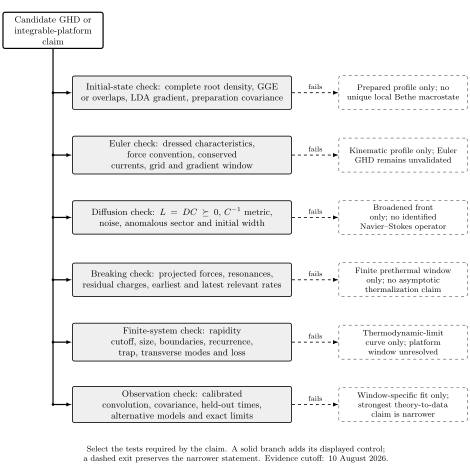
Validity map for theory-to-platform comparisons. Ideal Bethe or GHD equations become experimental predictions only after finite-system preparation and observation maps are included. Original schematic, not to scale; experimental evidence is bounded through 10 August 2026.

Benchmark and falsification design

Separate calibration, validation, and extrapolation:

1. Fix $c$, atom number, trap, temperature, initial state, resolution, and loss from independent data.
2. Test exact particle-number and energy constraints and an analytically controlled limit.
3. Compare several times and observables with a single parameter set and full covariance.
4. Vary system size, trap strength, interaction, and resolution to move suspected corrections predictably.
5. Compare Euler, diffusive, weak-breaking, and nonintegrable alternatives on held-out data.
6. State a no-validation result if agreement exists only after time-dependent refitting or window selection.

Schemmer, Bouchoule, Doyon, and Dubail 2019, main text and supplemental analysis compared one-dimensional Bose-gas expansion on an atom chip with GHD using independently characterized trapping and interactions. Malvania et al. 2021, main text and supplementary comparison tested GHD in a strongly interacting one-dimensional Bose gas over a broad dynamical protocol. These experiments validate specified observables and windows, not a platform-independent absence of integrability breaking.

Le et al. 2023, main text, Methods, and source data observed hydrodynamization and local prethermalization in one-dimensional Bose gases. The distinction in the title is important: local prethermal behavior can be well described before global thermalization, and the observation does not collapse those timescales into one.

The experimental and source assessment is current through 10 August 2026. Later platform data, revised calibrations, corrections, and disputed asymptotic claims belong in the Quantum Matter and Emergence Research synthesis. The canonical integrable-matter claim test matrix records the finite-size, breaking, and validation ceiling. A reproducible verification workflow performs finite-grid, convolution, and held-out-time tests.

Exercise

Resolution can mimic front broadening. Suppose an intrinsic front is approximately Gaussian with variance $w_{\mathrm{th}}^2(t)=2Dt$, and the calibrated imaging point-spread function is Gaussian with variance $\sigma_{\mathrm{img}}^2$. Find the observed variance. What goes wrong if one fits $w_{\mathrm{obs}}^2=2D_{\mathrm{fit}}t$ through the origin?

Solution

The convolution of two Gaussians adds variances:

$$w_{\mathrm{obs}}^2(t) =2Dt+\sigma_{\mathrm{img}}^2.$$

An origin-constrained fit attributes the fixed intercept to time-dependent diffusion, giving

$$D_{\mathrm{fit}}(t) =D+\frac{\sigma_{\mathrm{img}}^2}{2t}$$

for a single-time estimate. It overestimates diffusion most strongly at early times and creates an apparent time-dependent coefficient. A valid fit propagates the independently calibrated $\sigma_{\mathrm{img}}$ and its covariance, and also includes the initial physical width.

References

• Le, Y., Zhang, Y., Gopalakrishnan, S., Rigol, M., and Weiss, D. S. (2023). “Observation of hydrodynamization and local prethermalization in 1D Bose gases.” Nature 618, 494–499. doi:10.1038/s41586-023-05979-9.
• Malvania, N., Zhang, Y., Le, Y., Dubail, J., Rigol, M., and Weiss, D. S. (2021). “Generalized hydrodynamics in strongly interacting 1D Bose gases.” Science 373, 1129–1133. doi:10.1126/science.abf0147.
• Schemmer, M., Bouchoule, I., Doyon, B., and Dubail, J. (2019). “Generalized hydrodynamics on an atom chip.” Physical Review Letters 122, 090601. doi:10.1103/PhysRevLett.122.090601.