From Measured Intensity to Many-Body Claim

A many-body measurement is an inverse problem: the detector records counts, voltages, arrival times, or images, whereas the scientific claim concerns an operator correlation function, a model parameter, or a phase. A credible inference keeps every map between those levels explicit. The result is not merely a corrected spectrum; it is a statement whose normalization, uncertainty, alternatives, and domain of validity can be reconstructed from the raw record.

Required background. Correlator conventions fixes the response and spectral objects used below. Transport extraction and inverse errors supplies regularization, covariance, and inverse-problem language.

Evidence cutoff. This method and evidence account covers primary and official sources available through 10 August 2026. Later calibrations, corrections, datasets, and changing assessments belong in the dated Quantum Matter and Emergence Research synthesis.

The forward measurement model

Let $d_i$ be the recorded data in detector bin $i$. A useful common form is

$$d_i=b_i(\eta)+ \int d\lambda\,R_i(\lambda;\eta) M(\lambda;\eta)\,C(\lambda;\theta) +\epsilon_i.$$

$C$ is a normalized correlator or response predicted by the physical model with parameters $\theta$; $M$ contains matrix elements, form factors, efficiencies, and kinematic factors; $R_i$ is the resolution and binning kernel; $b_i$ is background; and $\eta$ collects calibration and nuisance parameters. The noise vector $\epsilon$ has covariance $\Sigma$, which generally is not diagonal after normalization, deconvolution, drift correction, or shared-background subtraction.

This equation is deliberately a forward map. Direct deconvolution can magnify small singular directions of $R$ and create sharp structures not supported by the data. Fitting a convolved candidate $RMC$ to $d$ preserves the experiment’s information content and makes regularization or prior dependence visible; Tarantola 2005, chs. 1–3 develops this inverse-theory viewpoint. The NIST uncertainty framework treats the measurement equation, input distributions, and output uncertainty as one object Possolo 2015, NIST TN 1900.

The chapter’s original structure diagram follows this map from left to right. Inspect the central rule: a result may move forward only after its normalization and uncertainty move with it.

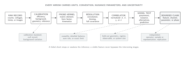
Measurement-to-claim structure. Each arrow is a documented transformation with nuisance parameters and uncertainty; none licenses a jump from a visible feature directly to a phase or mechanism. The diagram is schematic and not tied to one instrument.

Normalization, covariance, and identifiability

Normalization conditions are strong internal checks. A one-particle spectrum in this volume obeys

$$A(\mathbf k,\omega)=-2\,\operatorname{Im}G^R(\mathbf k,\omega), \qquad \int_{-\infty}^{\infty}\frac{d\omega}{2\pi} A(\mathbf k,\omega)=1,$$

while a structure factor integrates to the corresponding equal-time correlation in its stated Fourier convention. A fitted curve that violates a known sum rule has not been rescued by a small residual.

For Gaussian residuals $r=d-\mu(\theta,\eta)$,

$$-2\ln L=r^{\mathsf T}\Sigma^{-1}r+\ln\det\Sigma+\text{constant}.$$

Dropping off-diagonal covariance changes both parameter errors and model rankings. Near-singular $\Sigma$ should be treated with a declared eigencut or shrinkage model whose stability is tested, not silently inverted. Calibration parameters shared across bins or experiments belong in the joint likelihood rather than being added later as independent error bars.

Even perfect data need not identify every parameter. With Jacobian $J_{ia}=\partial\mu_i/\partial\theta_a$, the local information matrix $J^{\mathsf T}\Sigma^{-1}J$ exposes weak or degenerate parameter combinations. A posterior narrowed mainly by a prior is a prior-conditioned constraint, not a measurement of that direction.

From feature to conclusion

Different conclusions require different evidence:

• Observation: a reproducible feature exists in the calibrated observable.
• Identification: its operator, momentum, energy, polarization, or symmetry assignment survives alternatives.
• Parameter constraint: a declared forward model limits $\theta$ after nuisance marginalization.
• Mechanism comparison: competing models make distinguishable held-out predictions.
• Phase claim: defining order, topology, or long-range behavior survives size, temperature, resolution, and preparation limits.

A peak can identify an excitation without identifying its microscopic mechanism. A gap-like suppression can be caused by matrix elements, finite temperature, lifetime broadening, inhomogeneity, or background subtraction. A successful fit can constrain an effective self-energy without proving that one interaction generated it. Model discrepancy can also trade against physical parameters, as Kennedy and O’Hagan 2001 make explicit. The probe and computation claim test matrix records this ceiling for every route in the chapter.

A reproducible record

For each published inference, retain the raw or minimally processed data; detector mask and calibration versions; background and resolution models; units and Fourier conventions; complete covariance or resampling objects; priors and nuisance parameters; code and environment versions; failed or alternative fits; and the exact statement licensed by the result. The FAIR principles apply to workflows as well as data Wilkinson et al. 2016, but findability alone is not reproducibility: a second analyst must be able to regenerate the plotted observable and its uncertainty.

Exercise

Resolution-induced covariance. Two independent detector bins $x_1,x_2$ have variance $s^2$. A processed spectrum reports $y_1=x_1$ and $y_2=x_2-x_1$. Find the covariance of $y$ and explain why treating the two outputs as independent is wrong.

Solution

With

$$y=Ax, \qquad A=\begin{pmatrix}1&0\\-1&1\end{pmatrix}, \qquad \operatorname{Cov}(x)=s^2I,$$

the propagated covariance is

$$\operatorname{Cov}(y)=A(s^2I)A^{\mathsf T} =s^2\begin{pmatrix}1&-1\\-1&2\end{pmatrix}.$$

The shared $x_1$ makes the processed bins anticorrelated. A diagonal likelihood would overcount the shared information and generally distort both the fitted uncertainty and goodness of fit.

References

• Marc C. Kennedy and Anthony O’Hagan, “Bayesian Calibration of Computer Models,” Journal of the Royal Statistical Society B 63 (2001) 425–464. DOI
• Antonio Possolo, Simple Guide for Evaluating and Expressing the Uncertainty of NIST Measurement Results, NIST Technical Note 1900, 2015. DOI
• Albert Tarantola, Inverse Problem Theory and Methods for Model Parameter Estimation, SIAM, 2005. DOI
• Mark D. Wilkinson, Michel Dumontier, IJsbrand Jan Aalbersberg, Gabrielle Appleton, Myles Axton, Arie Baak, Niklas Blomberg, Jan-Willem Boiten, Luiz Bonino da Silva Santos, Philip E. Bourne, Jildau Bouwman, Anthony J. Brookes, Tim Clark, Mercè Crosas, Ingrid Dillo, Olivier Dumon, Scott Edmunds, Chris T. Evelo, Richard Finkers, Alejandra Gonzalez-Beltran, Alasdair J. G. Gray, Paul Groth, Carole Goble, Jeffrey S. Grethe, Jaap Heringa, Peter A. C. ’t Hoen, Rob Hooft, Tobias Kuhn, Ruben Kok, Joost Kok, Scott J. Lusher, Maryann E. Martone, Albert Mons, Abel L. Packer, Bengt Persson, Philippe Rocca-Serra, Marco Roos, Rene van Schaik, Susanna-Assunta Sansone, Erik Schultes, Thierry Sengstag, Ted Slater, George Strawn, Morris A. Swertz, Mark Thompson, Johan van der Lei, Erik van Mulligen, Jan Velterop, Andra Waagmeester, Peter Wittenburg, Katherine Wolstencroft, Jun Zhao, and Barend Mons, “The FAIR Guiding Principles for Scientific Data Management and Stewardship,” Scientific Data 3 (2016) 160018. DOI