One-Dimensional Quantum Matter

Particle ordering, two Fermi points, compact collective fields, and strong infrared fluctuations organize the one-dimensional models studied here. Generic interacting gapless liquids have spectral continua rather than a quasiparticle pole; the free-fermion limit retains its pole. This chapter builds a convention-complete route from lattice operators to Luttinger liquids, gapped sine–Gordon sectors, non-Abelian spin theories, spectral signatures, and boundary transport. Every result is tied to its charge lattice, symmetry, and regime of validity.

Helpful background. Jordan–Wigner Maps and the Lattice–Continuum Dictionary provides a direct diagnostic of lattice strings and continuum phases; Free Bosons and Vertex Operators provides the compact-boson correlators used throughout.

Enter this chapter

The local convention used throughout is

$$[\phi(x),\partial_y\theta(y)]=i\pi\delta(x-y), \qquad \rho-\rho_0=-\frac1\pi\partial_x\phi,$$

with spinless fermions

$$\psi_r=\frac{\eta_r}{\sqrt{2\pi a_0}}e^{-i(r\phi-\theta)}, \qquad H=\frac{u}{2\pi}\int dx \left[K(\partial_x\theta)^2+K^{-1}(\partial_x\phi)^2\right].$$

Consequently $e^{i(m\phi+n\theta)}$ has bulk dimension

$$\Delta_{m,n}=\frac14\left(m^2K+\frac{n^2}{K}\right).$$

The displayed symbols are not portable one at a time. A complete translation must carry the commutator, density, Hamiltonian, compactification, zero-mode lattice, and physical vertex operators together. The first diagram shows why both local and global data are needed.

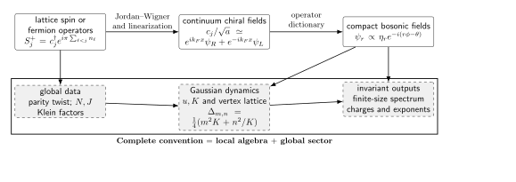
The one-dimensional dictionary has two inseparable parts: local operator bosonization and the global sector data that select physical states. The diagram is schematic; its equations use this chapter’s convention.

A route through the subject

Start with Jordan–Wigner Maps and the Lattice–Continuum Dictionary to transform spins, retain the parity-dependent closing bond, and linearize near $\pm k_F$. The Abelian Bosonization Dictionary fixes chiral vertices, densities, currents, and scaling dimensions. Zero Modes, Klein Factors, and Compactification completes the finite-size Hilbert space.

Luttinger Liquids develops the universal Gaussian fixed line identified by Haldane 1981, pp. 2585–2609 and the extraction of $u$ and $K$. Spinful and Multicomponent Luttinger Liquids separates charge, spin, and flavor modes while retaining their compact selection rules. Sine–Gordon Perturbations, Commensurability, and Duality determines when a symmetry-allowed vertex locks a field and how soliton charge follows from compactification.

Non-Abelian Bosonization and Spin Sectors replaces Abelian spin fields by affine currents and WZW primaries, following the critical spin-chain construction of Affleck 1986, pp. 409–447. Spin–Charge Separation and Spectral Observables translates sector factorization into spectral thresholds and probe-specific tests. Impurities, Junctions, and Transport in One Dimension treats the boundary flows derived by Kane and Fisher 1992, §§ II–IV, including weak barriers, weak links, leads, and multichannel conditions.

Convention and validity table

The Gaussian entries assume positive velocities and stiffnesses, $u>0$ and $K>0$ for each gapless mode, in the low-energy window where linearization applies. Bulk powers are zero-temperature, long-distance fixed-point results; marginal interactions, finite temperature, and finite size require their own corrections or crossovers. Allowed vertices must lie on the physical compactification lattice. “Relevant” refers to a weak perturbation at the stated bulk or boundary fixed point; a strong-coupling phase still requires symmetry and compactification checks.

Low-energy operator dimensions and their validity conditions. The comparison keeps local scaling data together with the global or boundary information needed to use them.

Object or claim	This chapter’s convention	Scaling statement	Global or boundary datum	Direct check	Failure if omitted
Smooth density	$\delta\rho=-\partial_x\phi/\pi$	derivative operator	$\phi(x+L)=\phi(x)-\pi N$	integrated charge is $N$	fractional or sign-reversed charge
Spinless fermion	$\psi_r\propto\eta_r e^{-i(r\phi-\theta)}$	$2\Delta_\psi=(K+K^{-1})/2$	Klein factors and parity twist	$K=1$ gives $1/x$	wrong interspecies signs or ring spectrum
General vertex	$V_{m,n}=e^{i(m\phi+n\theta)}$	$\Delta=(m^2K+n^2/K)/4$	$(m,n)$ must lie on the physical vertex lattice	charge, momentum, exchange phase	spurious local operators
Density locking	$\cos(2p\phi)$	bulk relevant for $p^2K<2$	commensurability and translation	kink charge magnitude $1/p$	a rapidly oscillating term is treated as a gap
Phase locking	$\cos(2q\theta)$	bulk relevant for $q^2/K<2$	charge symmetry must permit it	duality under $K\leftrightarrow K^{-1}$	simultaneous sharp locking of conjugate fields
Single spinless-channel backscattering	$\cos[2\phi(0)]$	boundary dimension $K$ at the transmitting fixed point	single channel; specified reservoirs and boundary conditions	two identical open ends: weak-link dimension $1/K$	bulk and boundary relevance are confused
Spinful electron	charge and spin vertices divided by $\sqrt2$	$\alpha_{\mathrm{bulk}}=(K_c+K_c^{-1}-2)/4$ for a gapless SU(2) spin fixed point	correlated charge–spin zero modes	free limit $K_c=1$	incorrect tunneling exponent
Spectral function	$A=-2\operatorname{Im}G^R$	generic interacting gapless thresholds; the free coincident-velocity limit has a pole	temperature, curvature, transverse hopping	$\int d\omega\,A/(2\pi)=1$ for the complete canonical fermion over all frequencies	intensity is mistaken for normalized spectral weight

The gapless spin qualification is essential: SU(2) symmetry alone does not exclude a spin gap Kane and Fisher 1992, § II, pp. 15236–15237. The weak-barrier and weak-link dimensions refer to the two stated spinless boundary fixed points, not a generic multichannel junction Kane and Fisher 1992, §§ III A–B, pp. 15238–15240. For the spectral row, $K_c=K_s=1$ and $u_c=u_s=v_F$ recover the free pole; a truncated low-energy spectral window need not carry unit weight.

Download the comparison data (JSON).

From an allowed operator to a physical claim

An RG eigenvalue is only the middle of the reasoning. First establish that the microscopic symmetries and compact vertex lattice allow the operator. Then distinguish bulk from boundary dimensions and declare the cutoff window. Finally test the predicted charge, finite-size sector, response normalization, and competing mechanism. The second diagram makes these decision points explicit.

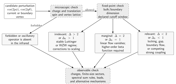
Symmetry and compactification can remove a candidate operator before scaling is considered. A relevant operator identifies an instability of the fixed point, not by itself the final strong-coupling phase; at $\Delta=2$ or $\Delta_b=1$, the linear flow vanishes and a higher-order beta function is required. The diagram is schematic and separates bulk from boundary thresholds.

Review the chapter

1. Starting from the Jordan–Wigner map, derive the sign cancellation that makes transverse spins commute on different sites and explain the periodic-chain parity twist.
2. Translate a bosonization formula written with $\rho=-\partial_x\widetilde\phi/\sqrt\pi$ into this chapter’s fields without changing a physical exponent.
3. Use finite-size charge and current energies to construct two independent measurements of $u$ and $K$.
4. Compare $\cos(4\phi)$ in a half-filled spinless fermion chain with $\cos(2\phi)$ for integer-filled bosons.
5. Explain why two spectral edges are stronger evidence for spin–charge separation when their velocities agree with charge and spin response measurements.
6. Reconcile the intrinsic $Ke^2/h$ response of a uniform spinless liquid with the $e^2/h$ two-terminal conductance of a wire attached to noninteracting leads.

References

• Affleck, I. “Exact Critical Exponents for Quantum Spin Chains, Nonlinear Sigma Models at $\theta=\pi$ and the Quantum Hall Effect.” Nuclear Physics B 265 (1986): 409–447. DOI.
• Haldane, F. D. M. “‘Luttinger Liquid Theory’ of One-Dimensional Quantum Fluids. I. Properties of the Luttinger Model and Their Extension to the General 1D Interacting Spinless Fermi Gas.” Journal of Physics C: Solid State Physics 14 (1981): 2585–2609. DOI.
• Kane, C. L., and M. P. A. Fisher. “Transmission through Barriers and Resonant Tunneling in an Interacting One-Dimensional Electron Gas.” Physical Review B 46 (1992): 15233–15262. DOI.

Further reading

• Giamarchi, T. Quantum Physics in One Dimension. Oxford: Clarendon Press, 2004. Publisher.