Eliashberg Equations and Retarded Pairing

Eliashberg theory keeps the frequency dependence that an exchanged phonon imprints on both the normal and anomalous electron self-energies. In the conventional isotropic problem, the functions $Z_n$ and $\Delta_n$ describe mass renormalization and pairing on fermionic Matsubara frequencies. Solving their coupled equations is a method, not a mechanism certificate: the preceding Migdal gate must control the omitted vertex corrections, the Coulomb sector must be matched without double counting, and numerical and analytic-continuation errors must be separated from physical assumptions.

This page derives the isotropic single-band equations, formulates $T_c$ as an eigenvalue problem, gives weak- and strong-coupling checks, and defines an auditable numerical workflow. Momentum anisotropy, multiband structure, strongly energy-dependent density of states, and vertex-complete theories require an enlarged method rather than silent changes to these equations.

Required background. Migdal validity supplies the noncrossing control condition. Nambu–Gor’kov propagators supplies the matrix self-energy and anomalous component.

Helpful background. Matsubara frequencies supplies thermal sums and continuation conventions.

The isotropic method begins with declared reductions

Use $\hbar=k_B=1$. The canonical equations below assume:

• a single, spin-degenerate band with a broad, approximately symmetric electronic window;
• an isotropic, even-frequency, spin-singlet $s$-wave state in a real gap gauge;
• a density of states that is effectively constant across the relevant phonon and pairing scales;
• particle–hole symmetry, so the energy-shift self-energy $\chi_n$ vanishes and no separate number equation is needed;
• an interaction represented by an isotropic electron–phonon spectrum $\alpha^2F(\Omega)$ and a separately matched Coulomb pseudopotential; and
• a previously validated Migdal approximation, with no material impurity, anisotropic, multiband, or competing-channel vertex omitted.

Before imposing particle–hole symmetry, write the Nambu inverse propagator as

$$\mathcal G^{-1}(\mathbf k,i\omega_n) =i\omega_nZ_n\tau_0 -[\xi_{\mathbf k}+\chi_n]\tau_3 -\phi_n\tau_1, \qquad \Delta_n\equiv\frac{\phi_n}{Z_n},$$

with fermionic frequencies $\omega_n=(2n+1)\pi T$. If $\chi_n$ is not negligible, it and the chemical potential or number equation must be solved; setting it to zero is a physical reduction, not notation.

In the Migdal approximation the phonon contribution to the Nambu self-energy has the schematic form

$$\hat\Sigma(\mathbf k,i\omega_n) =-T\sum_m\int_{\mathbf q} \lvert g_{\mathbf q}\rvert^2 D(\mathbf q,i\omega_n-i\omega_m) \tau_3\hat G(\mathbf k-\mathbf q,i\omega_m)\tau_3,$$

plus the screened Coulomb contribution in the anomalous channel. The overall sign is tied to the declared phonon-propagator convention; the physical kernel below fixes the normalization used here.

Fermi-surface averaging and the constant-density-of-states integral over $\xi$ reduce the momentum structure to

$$\lambda_{n-m} =2\int_0^\infty\mathrm d\Omega\, \frac{\Omega\,\alpha^2F(\Omega)} {\Omega^2+(\omega_n-\omega_m)^2}.$$

Its zero-transfer value defines

$$\lambda\equiv\lambda_0 =2\int_0^\infty\frac{\mathrm d\Omega}{\Omega} \alpha^2F(\Omega).$$

These equations also define the units of $\alpha^2F$: the final $\lambda$ is dimensionless.

Coupled mass and gap equations

For the reductions just stated, the all-integer Matsubara sums give

$$Z_n =1+\frac{\pi T}{\omega_n} \sum_{m=-\infty}^{\infty} \lambda_{n-m} \frac{\omega_m}{\sqrt{\omega_m^2+\Delta_m^2}},$$ $$Z_n\Delta_n =\pi T\sum_{m=-\infty}^{\infty} \left[ \lambda_{n-m} -\mu^\ast(\omega_c) \Theta(\omega_c-\lvert\omega_m\rvert) \right] \frac{\Delta_m}{\sqrt{\omega_m^2+\Delta_m^2}}.$$

An even-frequency solution satisfies the exact index relations

$$Z_{-n-1}=Z_n, \qquad \Delta_{-n-1}=\Delta_n,$$

because $\omega_{-n-1}=-\omega_n$. A symmetric numerical grid should preserve that pairing of indices rather than reconstruct it approximately.

There is no zero fermionic Matsubara frequency. The correct low-energy mass check is

$$\lim_{T\to0,\,\omega_n\to0^+}Z(i\omega_n)=1+\lambda$$

in the normal state under the same broad-band and constant-density-of-states assumptions. At high frequency, $Z_n\to1$ and the anomalous component decays. Marsiglio 2020, §II, Eqs. (3)–(21) derives the momentum-dependent and isotropic forms and their symmetry relations.

Three cutoffs perform three different jobs

A robust implementation names three scales separately.

1. $\Omega_{\max}$ is the physical upper support of the phonon spectrum.
2. $\omega_c$ is the physical matching scale at which the reduced Coulomb pseudopotential enters the low-energy equation.
3. $\omega_{\max,\mathrm{num}}$ is the numerical Matsubara truncation and must be taken to convergence.

For a regular broad electronic band of half-width $W/2$, a dimensionless Fermi-surface-projected repulsion $\mu$, and the hierarchy $\Omega_{\max}\ll\omega_c\ll W/2$, the Morel–Anderson reduction is

$$\mu^\ast(\omega_c) =\frac{\mu} {1+\mu\log[(W/2)/\omega_c]}.$$

If the matching scale changes, $\mu^\ast$ must change with it:

$$\frac{1}{\mu^\ast(\omega_{c,2})} =\frac{1}{\mu^\ast(\omega_{c,1})} +\log\frac{\omega_{c,1}}{\omega_{c,2}}.$$

Varying $\omega_c$ while holding $\mu^\ast$ fixed changes the physical model. By contrast, increasing $\omega_{\max,\mathrm{num}}$ should leave a converged low-energy solution unchanged. The reduction itself assumes a smooth density of states and screened interaction across the eliminated window; it is not automatic in a narrow, flat, multiband, or Mott-adjacent system. It must also not be combined with an independently retained microscopic Coulomb interaction over the same window. Morel and Anderson 1962, pp. 1263–1271 gives the original logarithmic matching.

The transition is an eigenvalue crossing

At $T_c$, first solve the normal-state renormalization

$$Z_n^N(T) =1+\frac{\pi T}{\omega_n} \sum_m\lambda_{n-m}\operatorname{sgn}\omega_m.$$

Then linearize the anomalous equation:

$$Z_n^N(T)\Delta_n =\pi T\sum_m \left[ \lambda_{n-m} -\mu^\ast(\omega_c) \Theta(\omega_c-\lvert\omega_m\rvert) \right] \frac{\Delta_m}{\lvert\omega_m\rvert}.$$

Write the right-hand side as a temperature-dependent matrix acting on $\Delta_m$. With a normalization in which its leading eigenvalue is $\rho(T)$,

$$\rho(T_c)=1.$$

Bracketing this crossing is numerically cleaner than searching for a vanishing nonlinear gap. The leading eigenvector also supplies a controlled initial shape for the nonlinear solution below $T_c$.

Einstein spectrum and analytic checks

For

$$\alpha^2F(\Omega) =\frac{\lambda\Omega_E}{2}\delta(\Omega-\Omega_E),$$

the kernel is

$$\lambda_{n-m} =\lambda\frac{\Omega_E^2} {\Omega_E^2+(\omega_n-\omega_m)^2},$$

so $\lambda_{n-n}=\lambda$ is an immediate normalization check.

The familiar hard-cutoff BCS reduction sets $Z=1$ and replaces the retarded kernel by a constant inside $\Omega_E$, giving

$$T_c^{\mathrm{static}} \simeq1.13\,\Omega_Ee^{-1/\lambda}.$$

That is a useful reduced-model check, but it is not the full prefactor of the retarded Einstein Eliashberg problem. For $\mu^\ast=0$ in the weak-coupling Einstein model,

$$T_c =\frac{1.13}{\sqrt e}\,\Omega_E \exp\!\left[-\frac{1+\lambda}{\lambda}\right],$$ $$\Delta_0 =\frac{2}{\sqrt e}\,\Omega_E \exp\!\left[-\frac{1+\lambda}{\lambda}\right],$$

while $2\Delta_0/T_c\to3.53$. The durable leading statement is $\log(\Omega_E/T_c)\sim1/\lambda$; the prefactor and constant in the exponent belong to the specified spectrum and convention. Mirabi, Boyack, and Marsiglio 2020, §III derives the $1/\sqrt e$ retarded correction.

At the opposite formal limit, the canonical isotropic equations with $\mu^\ast=0$ give

$$T_c\simeq0.1827\sqrt{\lambda\langle\Omega^2\rangle}, \qquad \lambda\langle\Omega^2\rangle =2\int_0^\infty\mathrm d\Omega\, \Omega\alpha^2F(\Omega).$$

For an Einstein spectrum this becomes $0.1827\,\Omega_E\sqrt\lambda$ Allen and Dynes 1975, pp. 905–922. It is an equation-level strong-coupling asymptote, not proof that a real phonon spectrum, lattice, and Fermi liquid remain stable as $\lambda\to\infty$.

A reproducible solver has acceptance criteria

The right panel of the figure separates the physical inputs, coupled solve, and validation loop. It also prevents the three cutoff scales from being collapsed into one symbol.

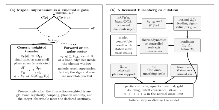
The canonical workflow begins only after the Migdal kinematic gate passes. The physical phonon support $\Omega_{\max}$, Coulomb matching scale $\omega_c$, and numerical cutoff $\omega_{\max,\mathrm{num}}$ enter different checks. A result is accepted only after symmetry, tail, equation-residual, grid, and cutoff-covariance tests; continuation and agreement with data still license model compatibility rather than mechanism proof. Original schematic, not to scale.

An implementable procedure is:

1. validate $\alpha^2F(\Omega)$, its units and nonnegativity where appropriate, $\lambda$, $\Omega_{\max}$, and the moments used later;
2. choose a symmetric grid $n=-N,\ldots,N-1$, so $\omega_{-n-1}=-\omega_n$ is represented exactly;
3. take $\omega_{\max,\mathrm{num}}$ well beyond both $\Omega_{\max}$ and $\omega_c$, while recording it separately from them;
4. build $\lambda_{n-m}$ and verify its symmetry and an analytic spectrum check such as $\lambda_{n-n}=\lambda$;
5. solve $Z_n^N$ and the linearized eigenproblem, bracket $\rho(T)-1$, and locate $T_c$;
6. below $T_c$, iterate the nonlinear equations with damping, Anderson mixing, or a Newton-like method;
7. report a normed equation residual—iteration count or a small update alone is not convergence;
8. double $N$ or $\omega_{\max,\mathrm{num}}$ and verify stability of $T_c$, $Z_n$, $\Delta_n$, and any derived observable;
9. vary $\omega_c$ while transforming $\mu^\ast$ covariantly and check low-energy invariance; and
10. verify even-frequency parity, high-frequency tails, the normal low-frequency $Z\to1+\lambda$ limit, and a weak- or strong-coupling benchmark only in its stated domain.

The method stops or expands if the Migdal gate fails, the density of states varies materially over the phonon window, the Coulomb scale separation is absent, anisotropy or several bands control the result, the phonon input is unstable, or the answer remains sensitive to a numerical or matching cutoff.

Real-axis observables are a second inverse problem

Three tasks should not be conflated:

• solving the forward Matsubara equations for a specified kernel;
• solving direct real-axis or mixed-representation equations for a specified kernel; and
• inferring $\alpha^2F$ from noisy tunnelling, optical, or thermodynamic data.

Analytic continuation from Matsubara values is ill-conditioned. A Padé approximant can be useful for exceptionally accurate smooth data, but its poles and zeros must be tested under precision and grid changes. When detailed spectra are central, direct real-axis or mixed-representation equations are usually safer. Any continuation should satisfy causality, Kramers–Kronig consistency, spectral positivity where applicable, known moments or sum rules, and back-evaluation at the original Matsubara points. Marsiglio 2020, §II.4 compares these interfaces.

On the real axis, complex $Z(\omega)$ and $\phi(\omega)$ generate mass shifts, lifetimes, gap-edge structure, and phonon features in tunnelling and optics. Distinct broadened spectra can nevertheless fit the same finite-resolution data. A credible inversion reports covariance, backgrounds, resolution, regularization, sensitivity to $\mu^\ast$, and held-out observables.

What the solution can claim

A converged isotropic Eliashberg solution establishes the consequences of its declared retarded kernel within a licensed noncrossing approximation. Agreement with several observables can support that model. It does not, by itself, prove that the inferred boson is microscopic, unique, or causally dominant.

Stronger mechanism inference needs independent momentum, isotope, pressure, impurity, intervention, and competing-order tests. Anisotropic or sign-changing pairing requires momentum- and orbital-resolved kernels and vertices; continue to unconventional pairing symmetries rather than inserting a sign-changing gap into the isotropic equations without a matching interaction.

The shared validity map keeps vertex control, retarded self-consistency, and mechanism evidence on separate branches.

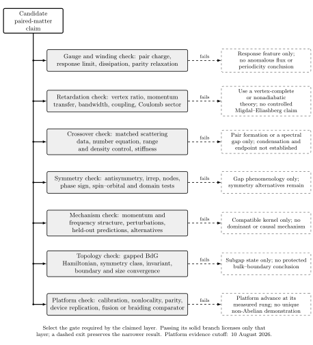
Passing the retardation branch licenses a controlled self-consistent kernel calculation under its stated assumptions. Passing it does not automatically pass the distinct mechanism branch. Failure of kernel normalization, Coulomb matching, continuation, or competing-model tests lowers the conclusion to compatibility with a restricted model or observable. Original schematic, not to scale.

The paired-matter claim test matrix states the corresponding evidence ceilings.

Common pitfalls

Writing $Z(0)=1+\lambda$ on a finite-temperature Matsubara grid. Fermionic frequencies never include zero. Take the normal-state $T\to0$, $\omega_n\to0^+$ limit or use the equivalent real-axis mass enhancement.

Using one symbol for every cutoff. Phonon support, Coulomb matching, and numerical truncation have different meanings. Only the numerical cutoff should disappear from a converged result.

Finding $T_c$ from a tiny nonlinear gap. Linearize about the normal solution and locate the leading-eigenvalue crossing. It supplies both a clean criterion and the gap shape at onset.

Calling a fitted $\alpha^2F$ the pairing mechanism. Inversion can be nonunique, and the assumed model has already excluded alternatives. Mechanism evidence must survive independent interventions and competing forward models.

Exercises

Einstein-kernel normalization

Evaluate $\lambda_{n-m}$ for the Einstein spectrum and find its zero-transfer value.

Solution

Substitution gives

$$\lambda_{n-m} =2\frac{\lambda\Omega_E}{2} \frac{\Omega_E}{\Omega_E^2+(\omega_n-\omega_m)^2} =\lambda\frac{\Omega_E^2} {\Omega_E^2+(\omega_n-\omega_m)^2}.$$

At $n=m$, it equals $\lambda$. This checks the spectrum’s coefficient, dimensions, and the definition of the dimensionless coupling.

Coulomb cutoff covariance

A calculation uses $\mu^\ast(10\Omega_E)=0.12$. What value represents the same low-energy repulsion if the matching scale is lowered to $5\Omega_E$?

Solution

Use

$$\frac1{\mu^\ast(5\Omega_E)} =\frac1{0.12}+\log\frac{10}{5}.$$

Thus

$$\mu^\ast(5\Omega_E) =\frac1{8.333+0.693} \simeq0.1108.$$

The lower matching scale integrates out a larger logarithmic interval and therefore reduces the residual repulsion. Keeping $0.12$ would define a different model.

Linearized transition matrix

On a finite symmetric grid, define

$$K_{nm}(T) =\frac{\pi T}{Z_n^N(T)} \left[ \lambda_{n-m}-\mu^\ast\Theta(\omega_c-\lvert\omega_m\rvert) \right] \frac1{\lvert\omega_m\rvert}.$$

Explain how to determine $T_c$ and give two convergence tests that must accompany it.

Solution

Compute the largest eigenvalue $\rho(T)$ of $K(T)$. At high temperature it is below one; on cooling it grows. Bracket temperatures with opposite signs of $\rho(T)-1$ and use bisection or a safeguarded root finder to solve $\rho(T_c)=1$.

At minimum, double the Matsubara range or $N$ and require $T_c$ to remain within the declared tolerance, and change $\omega_c$ while transforming $\mu^\ast$ by cutoff covariance. One should also verify the parity of the leading eigenvector and the residual norm $\lVert K\Delta-\Delta\rVert/\lVert\Delta\rVert$.

Static BCS versus retarded weak coupling

Compare the static hard-cutoff result with the weak-coupling Einstein expressions. Which prediction is unchanged at leading order?

Solution

The static model gives $T_c\simeq1.13\Omega_Ee^{-1/\lambda}$. The retarded Einstein solution retains frequency dependence in $Z$ and $\Delta$, producing a different constant prefactor and the exponent $(1+\lambda)/\lambda$. Both share the leading logarithm

$$\log\frac{\Omega_E}{T_c}\sim\frac1\lambda$$

as $\lambda\to0$. Because $T_c$ and $\Delta_0$ acquire the same retarded factor in this model, their ratio tends to the BCS value $2\Delta_0/T_c\simeq3.53$.

References

• Allen, P. B., and Dynes, R. C. (1975). “Transition temperature of strong-coupled superconductors reanalyzed.” Physical Review B 12, 905–922. doi:10.1103/PhysRevB.12.905.
• Allen, P. B., and Mitrović, B. (1983). “Theory of superconducting $T_c$.” Solid State Physics 37, 1–92. doi:10.1016/S0081-1947(08)60665-7.
• Carbotte, J. P. (1990). “Properties of boson-exchange superconductors.” Reviews of Modern Physics 62, 1027–1157. doi:10.1103/RevModPhys.62.1027.
• Eliashberg, G. M. (1960). “Interactions between electrons and lattice vibrations in a superconductor.” Soviet Physics JETP 11, 696–702. JETP archive.
• Marsiglio, F. (2020). “Eliashberg theory: A short review.” Annals of Physics 417, 168102. doi:10.1016/j.aop.2020.168102.
• Mirabi, S., Boyack, R., and Marsiglio, F. (2020). “Eliashberg theory in the weak-coupling limit: Results on the real frequency axis.” Physical Review B 101, 064506. doi:10.1103/PhysRevB.101.064506.
• Morel, P., and Anderson, P. W. (1962). “Calculation of the superconducting state parameters with retarded electron-phonon interaction.” Physical Review 125, 1263–1271. doi:10.1103/PhysRev.125.1263.