Model Selection and Parameter Inference

Many-body inference often compares several imperfect models using heterogeneous observables. Parameters of interest coexist with calibration and nuisance variables, numerical error, and structural model discrepancy. A best fit is therefore not a unique mechanism: model selection asks which predictive statements survive covariance, priors, discrepancy, identifiability, alternative hypotheses, and held-out data.

Required background. The measurement-to-claim map supplies the forward model. Transport extraction and inverse errors supplies regularization and uncertainty propagation.

Helpful background. Correlated fits and model selection supplies statistical stability tests.

Evidence cutoff. This method and evidence account covers primary and official sources available through 10 August 2026. Later statistical methods, corrections, datasets, and changing assessments belong in the dated Quantum Matter and Emergence Research synthesis.

A joint generative model

For data vector $y$ and candidate model $M$, write

$$y=f_M(\theta,\eta)+\delta_M(x)+\epsilon, \qquad \epsilon\sim\mathcal N(0,\Sigma_{\mathrm{exp}}+\Sigma_{\mathrm{num}}).$$

$\theta$ are physical parameters, $\eta$ are calibration and nuisance variables, $\delta_M$ represents structural discrepancy, and $\Sigma_{\mathrm{num}}$ propagates Monte Carlo, truncation, interpolation, or emulator error. The measurement-model construction and uncertainty propagation follow the framework of Possolo 2015, NIST TN 1900. For a Gaussian likelihood,

$$-2\ln L_M= r^{\mathsf T}\Sigma^{-1}r+\ln\det\Sigma+\text{constant}, \qquad r=y-f_M-\delta_M.$$

If different probes share sample geometry, energy calibration, Hamiltonian parameters, or background subtraction, their covariance is block structured rather than independent. Multiplying marginal likelihoods while omitting shared variables double counts information.

Structural discrepancy is not a free residual sponge. A highly flexible $\delta_M$ can absorb the same variation as $\theta$, destroying identifiability. Its scale and smoothness need physical justification and sensitivity tests; where no defensible discrepancy model exists, held-out predictive error should limit the conclusion explicitly. Kennedy and O’Hagan 2001 gives the foundational calibration formulation and its confounding structure.

The chapter validity figure shows model comparison after the probe and representation checks. Inspect the shared-assumption branch before treating several fitted observables as independent confirmation.

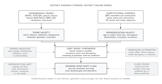
Model comparison within the evidence chain. A posterior or information criterion is conditional on its likelihood, priors, discrepancy, candidate set, and data-selection rule; predictive checks determine the strongest bounded conclusion. Schematic.

Identifiability and prior sensitivity

Local sensitivity is summarized by the Jacobian and its covariance-whitened form,

$$J_{ia}=\frac{\partial f_i}{\partial\theta_a}, \qquad J_{\mathrm w}=\Sigma^{-1/2}J, \qquad F=J_{\mathrm w}^{\mathsf T}J_{\mathrm w} =J^{\mathsf T}\Sigma^{-1}J.$$

Small eigenvalues of $F$ identify parameter combinations that the chosen observables barely constrain. Globally, multimodality and parameter symmetries can survive even when $F$ is nonsingular near one mode. Report profile likelihoods or posterior marginals, correlations, transformations, and predictions—not only optimizer errors.

Bayesian inference uses the conditioning rules and hierarchical structure developed systematically by Gelman et al. 2013:

$$p(\theta,\eta\mid y,M) \propto L(y\mid\theta,\eta,M) p(\theta,\eta\mid M).$$

The marginal likelihood $p(y\mid M)$ includes an Occam factor and can be strongly prior-volume dependent. Bayes factors therefore require scientifically justified proper priors and a sensitivity study. Frequentist likelihood ratios or information criteria have different regularity and candidate-set assumptions; agreement between criteria is useful but not a proof that the true mechanism is among the candidates.

Prediction before interpretation

Reserve data that were not used to choose preprocessing, parameter ranges, model variants, or discrepancy. Posterior predictive checks test whether simulated replicated data reproduce the features used in the claim. Leave-one-probe-out or leave-one-regime-out prediction is especially valuable when a model can interpolate each dataset separately.

For approximate leave-one-out comparison, pointwise expected log predictive density and its uncertainty are preferable to a bare rank. Vehtari, Gelman, and Gabry 2017 give stable diagnostics. If differences are comparable to their uncertainty or reverse under plausible priors, covariance, preprocessing, or discrepancy, the conclusion is model non-discrimination.

A mechanism claim should include at least one prediction that a plausible competitor does not share. A phase claim additionally requires a defining observable and its thermodynamic or topological limit. The probe and computation claim test matrix keeps likelihood, covariance, prior, nuisance treatment, discrepancy, candidate set, and held-out test together.

Exercise

A nonidentifiable product. Data obey $y_i=abx_i+\epsilon_i$ with known $x_i$ and Gaussian noise. Show why $a$ and $b$ cannot be separately identified from this dataset.

Solution

The mean depends only on $c=ab$. Its derivatives are $\partial_a f_i=bx_i$ and $\partial_b f_i=ax_i$, which are proportional columns of the Jacobian. Hence $F=J^{\mathsf T}\Sigma^{-1}J$ has rank one. The likelihood constrains $ab$ but is constant along the hyperbolas $ab=c$; separate posteriors for $a$ and $b$ are determined by priors or additional data.

References

• Andrew Gelman, John B. Carlin, Hal S. Stern, David B. Dunson, Aki Vehtari, and Donald B. Rubin, Bayesian Data Analysis, third edition, CRC Press, 2013. DOI
• Marc C. Kennedy and Anthony O’Hagan, “Bayesian Calibration of Computer Models,” Journal of the Royal Statistical Society B 63 (2001) 425–464. DOI
• Antonio Possolo, Simple Guide for Evaluating and Expressing the Uncertainty of NIST Measurement Results, NIST Technical Note 1900, 2015. DOI
• Aki Vehtari, Andrew Gelman, and Jonah Gabry, “Practical Bayesian Model Evaluation Using Leave-One-Out Cross-Validation and WAIC,” Statistics and Computing 27 (2017) 1413–1432. DOI