Competing Orders and Electronic Nematicity

Magnetic, charge, superconducting, and nematic orders can compete, coexist, or generate one another because they involve the same low-energy fermions. The central task is to separate three questions: which symmetry is broken, whether thermodynamic order forms, and what microscopic field drives it. A stable coupled-order theory answers the first two only within its declared regime; similar onset temperatures or anticorrelated intensities do not, by themselves, answer the third.

Required background. Use Pomeranchuk and density-wave distinctions and Hubbard symmetries. Helpful background. Functional RG compares weak-coupling channels.

Order parameters and the symmetries they break

An order parameter is defined by its transformation law, not by the probe that happens to detect it.

Stripe magnetism. The fields $\mathbf M_x$ at $\mathbf Q_x=(Q,0)$ and $\mathbf M_y$ at $\mathbf Q_y=(0,Q)$ break spin rotation and translation when their expectation values are nonzero; a single stripe also selects a lattice axis. Establishing it requires the magnetic structure factor, correlation length, ordered moment, domain population, and thermodynamic scaling.

Charge order. The complex amplitudes $\rho_x$ and $\rho_y$ at the same two wavevectors break translation and may also select an axis. A charge-order claim must state the wavevector and form factor and control the correlation length and probe matrix elements.

Superconductivity. A complex field $\Psi$ describes phase coherence in a neutral effective theory. In a charged system the gauge redundancy itself is not an ordinary spontaneously broken symmetry; gauge-invariant evidence comes from phase stiffness, Meissner response, and long-range or quasi-long-range pair correlations in the appropriate dimensional and temperature limit.

Primary nematicity. A uniform fermion bilinear $n_\Gamma$ breaks a point-group rotation, commonly $C_4\to C_2$, while preserving translation. Evidence requires a zero-strain response, spontaneous-domain and finite-size tests, and an explicit crystal-axis convention.

Vestigial nematicity. A composite such as $M_x^2-M_y^2$ or $|\rho_x|^2-|\rho_y|^2$ can break the same point-group symmetry while the finite-wavevector parent fields remain disordered. Establishing this mechanism requires both composite scaling and the predicted short-range parent correlations, not merely the shared broken symmetry.

A uniform nematic variable transforms in a nontrivial one-dimensional representation of the point group. With axes along square-lattice bonds, $x^2-y^2$ is conventionally called $B_{1g}$ and $xy$ is $B_{2g}$; rotating the axes by forty-five degrees interchanges those names. A quarter turn exchanges the two nematic domains and reverses the sign of either basis function. Naming the crystallographic axes and unit cell is therefore part of the definition.

Use an extensive operator and its intensive density distinctly:

$$\begin{aligned} \mathcal N_\Gamma &=\sum_{\mathbf k\sigma}f_\Gamma(\mathbf k) c^\dagger_{\mathbf k\sigma}c_{\mathbf k\sigma},\\ n_\Gamma&=\frac{\mathcal N_\Gamma}{V}. \end{aligned}$$

Convenient square-lattice basis functions are

$$\begin{aligned} f_{B_{1g}}(\mathbf k)&=\cos k_x-\cos k_y,\\ f_{B_{2g}}(\mathbf k)&=\sin k_x\sin k_y. \end{aligned}$$

The continuum $q=0$ Pomeranchuk bilinear and its collective dynamics are developed by Oganesyan, Kivelson, and Fradkin 2001, Eq. (1), pp. 195109-1–2. Electronic liquid-crystal taxonomy is due to Kivelson, Fradkin, and Emery 1998, pp. 550–553. A primary field $n_\Gamma$ and a vestigial composite $\phi$ may transform identically, so a term $\lambda_{n\phi}n_\Gamma\phi$ is symmetry allowed and the observed order is generally a mixture Fernandes et al. 2012, Eqs. (74)–(76), p. 024534-24. Symmetry alone cannot reveal which microscopic field is primary.

The figure separates the microscopic objects that produce the same broken lattice symmetry: inspect whether the parent field carries zero momentum or whether finite momenta cancel only in a composite.

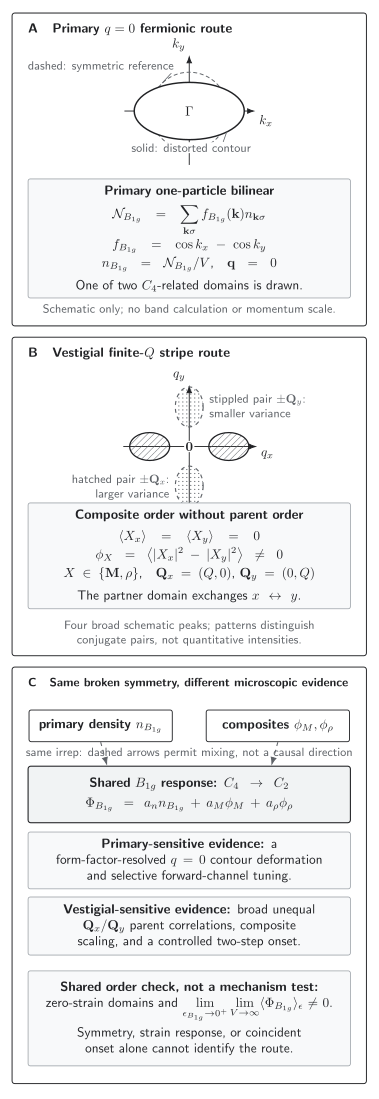
Primary and vestigial routes to the same bond-axis $B_{1g}$ nematic symmetry. A $q=0$ fermion bilinear directly distorts a $C_4$-symmetric Fermi contour, whereas unequal short-range stripe fluctuations generate the uniform composite $\phi=\langle M_x^2-M_y^2\rangle$ even when neither stripe amplitude orders. A ninety-degree rotation reverses either nematic domain, and symmetry permits the two fields to mix. The schematic is not to scale and does not identify the microscopic cause; distinguishing the routes requires comparing the $q=0$ form-factor response with finite-$Q$ parent correlations in the zero-strain thermodynamic limit.

The machine-readable figure record preserves the equations, arrow meanings, diagnostics, assumptions, and nonclaims without relying on vision.

Stripe magnetism, nematicity, and superconductivity

Magnetic and vestigial sectors

The subscripts in $\mathbf M_x$ and $\mathbf M_y$ label the ordering wavevectors, not spin components. A bond-axis quarter turn exchanges $\mathbf Q_x$ and $\mathbf Q_y$, so

$$\begin{aligned} S&=M_x^2+M_y^2 &&\text{is even},\\ \phi&=M_x^2-M_y^2 &&\text{is odd}, \end{aligned}$$

where $M_a^2=\mathbf M_a\!\cdot\!\mathbf M_a$. The source $h_\phi$ must transform like $\phi$; consequently $-h_\phi\phi$ is explicit symmetry breaking. Take all order-parameter amplitudes below to be intensive and write the uniform free-energy density as

$$\begin{aligned} f={}&\frac r2S+\frac u4S^2-\frac g4\phi^2-h_\phi\phi\\ &+r_\Psi|\Psi|^2+u_\Psi|\Psi|^4\\ &+w|\Psi|^2S. \end{aligned}$$

The real spin vectors displayed here are appropriate when each ordering wavevector is self-conjugate modulo a reciprocal lattice vector, $2\mathbf Q=\mathbf G$. For complex amplitudes define $S=|\mathbf M_x|^2+|\mathbf M_y|^2$ and $\phi=|\mathbf M_x|^2-|\mathbf M_y|^2$, but then the displayed $S,\phi$ functional is only a restricted amplitude sector. Invariants such as $|\mathbf M_a\!\cdot\!\mathbf M_a|^2$, inter-wavevector contractions, and commensurate Umklapp terms may also occur and can distinguish collinear, helical, and different double-$Q$ states.

Because $|\phi|\le S$, the magnetic quartic

$$q_4=\frac14\left(uS^2-g\phi^2\right)$$

is nonnegative for all magnetic configurations exactly when $u\ge0$ and $u-g\ge0$. It is strictly stabilizing in every nonzero direction when both inequalities are strict. On either equality boundary the quartic truncation has a flat direction, and a negative quadratic coefficient requires sixth-order or other stabilizing terms.

At fixed $S$, $g>0$ favors a single-$Q$ stripe with either $M_x\ne0$ or $M_y\ne0$, whereas $g<0$ favors an equal-amplitude double-$Q$ state with $\phi=0$. An additional invariant such as $(\mathbf M_x\!\cdot\!\mathbf M_y)^2$ is needed to decide whether two real double-$Q$ spin vectors are collinear or orthogonal. The composite $\phi$ is invariant under spin rotation, translation, and time reversal but changes sign under the quarter turn, so fluctuations can produce

$$\begin{aligned} \langle\phi\rangle &=\langle M_x^2-M_y^2\rangle\ne0,\\ \langle\mathbf M_x\rangle &=\langle\mathbf M_y\rangle=0. \end{aligned}$$

This is a vestigial Ising-nematic phase. In a strictly two-dimensional short-range system with exact continuous spin-rotation symmetry, magnetic long-range order is forbidden at nonzero temperature, while the discrete Ising nematic symmetry may still break Mermin and Wagner 1966, pp. 1133–1136. Weak interlayer coupling or spin anisotropy can restore a finite-temperature magnetic transition. An intermediate nematic regime is therefore symmetry allowed, not guaranteed. In a specific itinerant model, the preemptive regimes depend on dimension, elastic coupling, and generated coefficients Fernandes et al. 2012, Eq. (14), p. 024534-6, and Fig. 1 with §§ III.A–C, pp. 024534-8–20.

Competition with superconductivity

The pure superconducting sector requires $u_\Psi>0$. The sign of $w$ gives the local mean-field tendency: $w>0$ penalizes simultaneous magnetic amplitude and pairing, whereas $w<0$ favors them together. This coefficient does not replace the gauge-invariant superconducting evidence described above.

In the single-$Q$ sector set

$$\begin{aligned} x&=M_x^2\ge0,\\ y&=|\Psi|^2\ge0. \end{aligned}$$

Then

$$\begin{aligned} f(x,y)={}&\frac r2x+\frac{u-g}{4}x^2\\ &+r_\Psi y+u_\Psi y^2+wxy. \end{aligned}$$

Define $D=(u-g)u_\Psi-w^2$. Solving both stationarity equations gives

$$\begin{aligned} x_*&=\frac{-u_\Psi r+w r_\Psi}{D},\\ y_*&=\frac{wr-(u-g)r_\Psi}{2D}. \end{aligned}$$

A locally stable homogeneous mixed point requires $u-g>0$, $D>0$, $x_*>0$, and $y_*>0$; the determinant condition alone does not place the solution in the physical quadrant. For $w<0$, global boundedness on $x,y\ge0$ also requires $w>-\sqrt{(u-g)u_\Psi}$. Positive $w>\sqrt{(u-g)u_\Psi}$ leaves the quartic bounded on the physical quadrant but makes the mixed point unstable, producing competing pure phases or a first-order boundary at this order. This criterion is the page’s normalization of the standard two-order Ginzburg–Landau test Fernandes and Schmalian 2010, Eqs. (2)–(4), pp. 014521-3–4. Gradients, gauge fields, fluctuations, disorder, and higher-order terms can change this local uniform classification.

Charge-order couplings

Charge order enters by the same symmetry logic. Its composite

$$\phi_\rho=|\rho_x|^2-|\rho_y|^2$$

can mix linearly with $n_\Gamma$ and $\phi$ when all three belong to the same point-group representation. Terms such as $\lambda_{\rho\Psi}|\rho|^2|\Psi|^2$ describe local competition or cooperation. For a wavevector with $2\mathbf Q\not\equiv0$ modulo a reciprocal lattice vector, momentum conservation can also permit

$$\rho_{2\mathbf Q}^{*} \,\mathbf M_{\mathbf Q}\!\cdot\!\mathbf M_{\mathbf Q} +\mathrm{c.c.}$$

and thereby relate a spin modulation to a charge harmonic Nie et al. 2017, Eqs. (2.1)–(2.3), (2.10), and (4.1)–(4.2), pp. 085142-2–5. When $2\mathbf Q=\mathbf G$, the same contraction instead couples to a uniform scalar. Every allowed term must be derived from wavevectors and representations; shared symmetry or coincident onsets do not determine which field is primary.

Quantum susceptibility is an imaginary-time integral

Susceptibility is useful because a soft eigenvector reveals which normalized combination of coupled fields responds most strongly. It is not, by itself, a mechanism label.

Static thermodynamic response

Let

$$H(\mathbf h)=H_0-\sum_jh_jO_j,$$

where each source-independent $O_j$ is extensive, $h_j$ is its conjugate intensive field, and $\delta O_i=O_i-\langle O_i\rangle$. The isothermal equilibrium susceptibility is the zero-Matsubara-frequency Kubo correlation

$$\begin{aligned} \chi^T_{ij} &=\frac1V\frac{\partial\langle O_i\rangle}{\partial h_j}\\ &=\frac1V\int_0^\beta\!\mathrm d\tau\, \langle\delta O_j(\tau)\delta O_i(0)\rangle\\ &=\frac1V\int_0^\beta\!\mathrm d\tau\, \langle\delta O_i(\tau)\delta O_j(0)\rangle. \end{aligned}$$

Equilibrium cyclicity gives the two integral orderings and makes the symmetry of the free-energy Hessian explicit. If $O_i$ itself depends on $h_j$, its explicit derivative supplies an additional contact term. The companion page on sources and Kubo formulae develops the general response framework; the exact isothermal identity is Kubo 1957, Eq. (3.16), p. 576.

Whenever the source operator is imaginary-time independent—for example, when it commutes with $H_0$—the integral reduces to

$$\chi^T_{ij}=\frac{\beta}{V} \langle\delta O_j\delta O_i\rangle.$$

The same reduction holds in a classical commuting description; accidental special cases may also agree. For a generic quantum order parameter, however, replacing the imaginary-time integral by $\beta$ times an equal-time covariance can give the wrong magnitude and temperature dependence.

Matsubara and retarded response

Equilibrium simulations commonly evaluate discrete imaginary-frequency response, whereas an experiment measures causal real-time response. The Matsubara object is

$$\begin{aligned} \chi^M_{ij}(\mathbf q,i\omega_n) =\frac1V\int_0^\beta\!\mathrm d\tau\, e^{i\omega_n\tau} \langle T_\tau\delta O_i(\mathbf q,\tau) \delta O_j(-\mathbf q,0)\rangle. \end{aligned}$$

For the perturbation $-h_jO_j$, define

$$\begin{aligned} R_{ij}(\mathbf q,t) =\frac{i}{V}\theta(t) \langle[O_i(\mathbf q,t),O_j(-\mathbf q,0)]\rangle, \end{aligned}$$

so $\delta\langle O_i\rangle=R_{ij}*h_j$ and analytic continuation of $\chi^M$ gives $R$ with this sign convention. If zero-frequency modes equilibrate, the relevant ergodicity conditions hold, and the static continuation is regular, the thermodynamic response follows the static path

$$\chi^T_{ij} =\lim_{\mathbf q\to0}\lim_{\omega\to0} R_{ij}(\mathbf q,\omega).$$

Without equilibration, Kubo’s isolated or adiabatic static response can differ from the isothermal susceptibility even after an apparently regular $\omega\to0$ limit Kubo 1957, Eqs. (3.15)–(3.26), pp. 576–577. Taking the homogeneous limit first can also change the answer for conserved quantities, transport coefficients, or slow collective modes. A zero-Matsubara susceptibility and a low-frequency measurement are therefore not interchangeable without the limit path and relaxation assumptions.

Mixed susceptibility channels

For several orders, $\chi^T_{ij}$ is a real symmetric matrix. In the unbroken phase, off-diagonal mixing is restricted to operators in the same symmetry block. Its entries depend on the normalization of both operators and sources, so raw matrices from different bases are not directly comparable. A size-diverging eigenvalue—equivalently a vanishing eigenvalue of $(\chi^T)^{-1}$ after fixing normalization—supports an instability in the associated mixed channel; it does not identify whether that channel is primary, composite, electronic, or lattice assisted. At finite frequency, the retarded matrix is generally complex, and its poles or dynamical eigenmodes replace this static thermodynamic criterion.

Correlated estimates must retain the full covariance. Resample the underlying joint measurements, reconstruct the entire matrix in each bootstrap or jackknife replicate, and diagonalize each replicate; fitting entries and eigenvalues independently loses the correlations that determine the soft direction.

Strain, probes, and thermodynamic limits

Fixed strain

Nematic order couples linearly to strain in the same point-group representation. With the tensor-strain convention

$$\begin{aligned} \epsilon_{B_{1g}}&=\frac{\epsilon_{xx}-\epsilon_{yy}}{2},\\ \epsilon_{B_{2g}}&=\epsilon_{xy}, \end{aligned}$$

the engineering shear is $2\epsilon_{xy}$; changing convention rescales the associated modulus and coupling. For a generic intensive electronic nematic variable $\varphi_\Gamma$, the uniform, static, harmonic free-energy density is

$$\begin{aligned} f_{\mathrm{el}}={}&f_e(\varphi_\Gamma) +\frac{C_{\Gamma,0}}2\epsilon_\Gamma^2\\ &-\lambda_\Gamma\epsilon_\Gamma\varphi_\Gamma -\sigma_\Gamma\epsilon_\Gamma. \end{aligned}$$

Under imposed strain, $h_\varphi=\lambda_\Gamma\epsilon_\Gamma$ is a conjugate field: it selects a domain and rounds an Ising singularity. If the electronic sector equilibrates at each strain, its clamped-lattice susceptibility $\chi_e$ softens the measured uniform modulus to

$$C_\Gamma=C_{\Gamma,0}-\lambda_\Gamma^2\chi_e.$$

An elastoresistive slope is not automatically this thermodynamic susceptibility. For the symmetry-matched transport anisotropy $R_\Gamma=(\Delta\rho/\rho)_\Gamma$,

$$\begin{aligned} m_\Gamma &=\frac{\mathrm dR_\Gamma}{\mathrm d\epsilon_\Gamma}\\ &=\left(\frac{\partial R_\Gamma}{\partial\varphi_\Gamma}\right)_{\epsilon} \lambda_\Gamma\chi_e +\left(\frac{\partial R_\Gamma}{\partial\epsilon_\Gamma}\right)_{\varphi}. \end{aligned}$$

The first factor is a possibly parameter-dependent transport vertex; the second term is a regular direct piezoresistive background. The identification is therefore restricted to the linear near-zero-strain regime after controlling built-in strain and backgrounds Chu et al. 2012, Eqs. (1)–(4), pp. 710–712; Shapiro et al. 2015, Table II and Eqs. (17a)–(17b), pp. 235147-6–7.

Fixed stress

At fixed zero stress, minimizing over the relaxed strain gives

$$\epsilon_\Gamma =\frac{\lambda_\Gamma}{C_{\Gamma,0}}\varphi_\Gamma$$

and hence

$$\left(\chi_{\mathrm{eff}}\right)^{-1} =\chi_e^{-1}-\frac{\lambda_\Gamma^2}{C_{\Gamma,0}}.$$

The lattice thus shifts the transition and mixes electronic and structural response; imposed strain and fixed stress are different ensembles Fernandes et al. 2010, Eqs. (1), (2), and (5), pp. 157003-1–3; Chu et al. 2012, Eqs. (1)–(3), pp. 710–711. These scalar relations apply to uniform static response. At finite momentum, elastic compatibility produces a nonlocal anisotropic kernel. Long-range elasticity can then change the asymptotic critical theory Paul and Garst 2017, Eq. (2) and Figs. 2 and 4, pp. 227601-1–4.

Spontaneous order on finite systems

The normalized spontaneous nematic density is

$$n_{\Gamma,0} =\lim_{h_\Gamma\to0^+}\lim_{V\to\infty} \frac{\langle\mathcal N_\Gamma\rangle_{h_\Gamma}}{V} \ne0.$$

At exactly zero source, a finite symmetric system instead has $\langle\mathcal N_\Gamma\rangle=0$ even in an ordered regime. Its even moments retain the information. For a scalar Ising nematic define

$$\begin{aligned} S_N(0;L)&=\frac{\langle\mathcal N_\Gamma^2\rangle}{V},\\ m_N^2(L)&=\frac{S_N(0;L)}{V} =\frac{\langle\mathcal N_\Gamma^2\rangle}{V^2},\\ U_4(L)&=1- \frac{\langle\mathcal N_\Gamma^4\rangle} {3\langle\mathcal N_\Gamma^2\rangle^2}. \end{aligned}$$

True long-range order gives $m_N^2(L)\to n_{\Gamma,0}^2$ along a controlled sequence. Binder crossings and susceptibility peaks are finite-size estimators, not thermodynamic conclusions: fix the aspect ratio, boundary conditions, temperature or ground-state scaling, operator normalization, and leading corrections Binder 1981, pp. 119–140. The sibling sign-free QMC page derives a covariance-aware crossing workflow that applies to any appropriately defined dimensionless ratio.

A uniform source $h_\Gamma$ and quenched random strain $h_\Gamma(\mathbf r)$ are different problems. For random strain, state its distribution and correlation length, average disorder explicitly, and declare the order of disorder averaging, $V\to\infty$, and $h_\Gamma\to0$. A uniform-field extrapolation cannot recover a clean spontaneous intercept from an uncontrolled random-field domain pattern. Residual uniform strain, domain pinning, and unequal detector response can likewise imitate a nonzero intercept.

Evidence protocol and causal limits

The chapter validity map keeps a converged response separate from a mechanism attribution, and the claim table lists the shared covariance and competing-explanation checks.

1. Define each field. Give its wavevector, form factor, spin or orbital content, extensive or intensive normalization, and broken symmetry.
2. Establish the response. Use the full Kubo susceptibility or an equivalent derivative, with volume, temperature, boundaries, limit order, contacts, and covariance controlled. Reconstruct and diagonalize a susceptibility matrix inside each joint resample.
3. Establish order. Demonstrate correction-aware thermodynamic scaling, stiffness, or a long-range correlator. A broad maximum or one finite-size crossing is not an ordered phase.
4. Separate explicit, random, and spontaneous symmetry breaking. Extrapolate uniform strain or stress and domain imbalance in the correct order; treat quenched random strain with its own disorder average and limits.
5. Test coexistence microscopically. Follow region-resolved joint distributions or spatial cross-correlations and their finite-size scaling. An interior peak of a distribution built only from global amplitudes is not sufficient, because a phase-separated configuration can make both global intensities nonzero. Homogeneous coexistence requires thermodynamic weight for both orders in the same microscopic region or pure phase and an explicit exclusion of segregation; axis peaks or separated domains do not pass this test.
6. Bound causality. Compare primary and vestigial models, tune a selective control where possible, and predict a discriminating observable. Coincident onsets and spectral anticorrelation establish neither direction of cause.

Intertwined order is a useful organizing description even when no unique hierarchy survives these tests.

Common pitfalls

Using equal-time covariance as a quantum susceptibility. The static response is an imaginary-time integral in general. Check the operator dynamics before multiplying an equal-time fluctuation by $\beta$.

Calling strain a neutral probe. Symmetry-matched strain is a conjugate field and changes the electronic Hamiltonian. State the mechanical ensemble, transport vertex, background, and zero-strain extrapolation.

Inferring mechanism from shared symmetry. Primary Pomeranchuk and vestigial magnetic or charge composites can all produce the same nematic representation and may mix. Require both the $q=0$ response and finite-$Q$ parent-correlation tests.

Averaging domains into coexistence. Simultaneous bulk signals may come from mutually exclusive regions or Monte Carlo sectors. Use joint distributions, local probes, or spatial correlations before claiming homogeneous coexistence.

Promoting one finite-size feature to a phase boundary. A crossing or peak drifts with irrelevant corrections and geometry. Fit a controlled size sequence and propagate covariance.

Exercises

Explain how $\langle\phi\rangle\ne0$ can coexist with $\langle\mathbf M_x\rangle=\langle\mathbf M_y\rangle=0$.

Solution

$\phi=M_x^2-M_y^2$ is invariant under spin rotations but odd under the lattice operation exchanging $x$ and $y$. Fluctuations can choose unequal variances,

$$\langle M_x^2\rangle\ne\langle M_y^2\rangle,$$

without choosing a spin direction. Point-group symmetry is then broken while spin rotation and translation remain unbroken: this is vestigial nematic order.

Derive the local stability criterion for a homogeneous single-$Q$ magnetic and superconducting coexistence state.

Solution

For $x=M_x^2$ and $y=|\Psi|^2$, the Hessian of $f(x,y)$ is

$$\mathcal H= \begin{pmatrix} (u-g)/2 & w\\ w & 2u_\Psi \end{pmatrix}.$$

It is positive definite when its first diagonal entry and determinant are positive. Thus $u-g>0$ and $D=(u-g)u_\Psi-w^2>0$. Solving the stationarity equations gives

$$\begin{aligned} x_*&=\frac{-u_\Psi r+w r_\Psi}{D},\\ y_*&=\frac{wr-(u-g)r_\Psi}{2D}. \end{aligned}$$

Both values must be positive. For negative $w$, global boundedness additionally requires $w>-\sqrt{(u-g)u_\Psi}$; a positive competitive $w$ can leave the physical quadrant bounded even when the mixed stationary point is unstable.

Use $H_0=\Delta\sigma_z/2$ with $\Delta>0$ and a perturbation $-h\sigma_x$ to show why equal-time covariance is not generally the quantum susceptibility.

Solution

The positive eigenenergy is $E_h=\sqrt{(\Delta/2)^2+h^2}$, so the perturbed level splitting is $2E_h$. Thermal alignment with the Hamiltonian gives

$$\langle\sigma_x\rangle_h =\frac{h}{E_h}\tanh(\beta E_h).$$

Therefore

$$\begin{aligned} \chi^T_{xx} &=\left.\frac{\partial\langle\sigma_x\rangle_h}{\partial h}\right|_{h=0}\\ &=\frac{2}{\Delta} \tanh\left(\frac{\beta\Delta}{2}\right), \end{aligned}$$

whereas $\beta\langle(\delta\sigma_x)^2\rangle=\beta$ because $\sigma_x^2=1$. They agree only in the high-temperature limit $\beta\Delta\ll1$. If instead the source operator commutes with $H_0$, its imaginary-time correlator is constant and the Kubo integral reduces to $\beta$ times the equal-time covariance.

Compare the nematic response at fixed zero stress with the elastic response at imposed strain.

Solution

Write the electronic free-energy density to quadratic order as $f_e=\varphi^2/(2\chi_e)$. At fixed zero stress, stationarity gives $\epsilon=\lambda\varphi/C_0$. Substitution yields

$$\chi_{\mathrm{eff}}^{-1} =\chi_e^{-1}-\frac{\lambda^2}{C_0}.$$

At imposed strain, minimizing over $\varphi$ instead gives $\varphi=\lambda\chi_e\epsilon$ and

$$C=C_0-\lambda^2\chi_e.$$

The first result is a relaxed-lattice nematic susceptibility; the second gives the electronically softened uniform elastic modulus. They answer different mechanical boundary conditions.

A strained finite sample shows a growing transport anisotropy, broad magnetic peaks near $\mathbf Q_x$ that are stronger than those near $\mathbf Q_y$, no magnetic Bragg peak, and an increasing nematic susceptibility on cooling. What is established, what remains unproved, and which tests distinguish a primary from a vestigial mechanism?

Solution

The observations establish a strain-induced nematic response and anisotropic short-range stripe correlations. The absence of a Bragg peak is consistent with disordered magnetic parents, so the data are compatible with vestigial nematicity. They do not yet establish spontaneous order, exclude a primary $q=0$ field, or prove that the stripe fluctuations cause the anisotropy: strain already supplies a conjugate field, and the transport slope contains a vertex and a regular background.

First extrapolate the uniform strain to zero and control random strain and domains. Then test $m_N^2(L)$, $U_4(L)$, and the full Kubo susceptibility along a correction-aware size sequence, preserving covariance. Compare the scaling and selective tuning of the $q=0$ form-factor response with the finite-$Q$ parent correlations. A vestigial account becomes stronger only if one common model and parameter set explains both sectors and survives these zero-strain thermodynamic tests.

References

• Kurt Binder, “Finite Size Scaling Analysis of Ising Model Block Distribution Functions,” Zeitschrift für Physik B Condensed Matter 43 (1981) 119–140, doi:10.1007/BF01293604.
• Jiun-Haw Chu, Hsueh-Hui Kuo, James G. Analytis, and Ian R. Fisher, “Divergent Nematic Susceptibility in an Iron Arsenide Superconductor,” Science 337 (2012) 710–712, doi:10.1126/science.1221713.
• Rafael M. Fernandes, Andrey V. Chubukov, Johannes Knolle, Ilya Eremin, and Jörg Schmalian, “Preemptive Nematic Order, Pseudogap, and Orbital Order in the Iron Pnictides,” Physical Review B 85 (2012) 024534, doi:10.1103/PhysRevB.85.024534; erratum, Physical Review B 85 (2012) 109901, doi:10.1103/PhysRevB.85.109901.
• Rafael M. Fernandes and Jörg Schmalian, “Competing Order and Nature of the Pairing State in the Iron Pnictides,” Physical Review B 82 (2010) 014521, doi:10.1103/PhysRevB.82.014521.
• Rafael M. Fernandes, L. H. VanBebber, S. Bhattacharya, P. Chandra, V. Keppens, D. Mandrus, M. A. McGuire, B. C. Sales, A. S. Sefat, and J. Schmalian, “Effects of Nematic Fluctuations on the Elastic Properties of Iron Arsenide Superconductors,” Physical Review Letters 105 (2010) 157003, doi:10.1103/PhysRevLett.105.157003.
• Steven A. Kivelson, Eduardo Fradkin, and Victor J. Emery, “Electronic Liquid-Crystal Phases of a Doped Mott Insulator,” Nature 393 (1998) 550–553, doi:10.1038/31177.
• Ryogo Kubo, “Statistical-Mechanical Theory of Irreversible Processes. I. General Theory and Simple Applications to Magnetic and Conduction Problems,” Journal of the Physical Society of Japan 12 (1957) 570–586, doi:10.1143/JPSJ.12.570.
• N. David Mermin and Herbert Wagner, “Absence of Ferromagnetism or Antiferromagnetism in One- or Two-Dimensional Isotropic Heisenberg Models,” Physical Review Letters 17 (1966) 1133–1136, doi:10.1103/PhysRevLett.17.1133.
• Laimei Nie, Akash V. Maharaj, Eduardo Fradkin, and Steven A. Kivelson, “Vestigial Nematicity from Spin and/or Charge Order in the Cuprates,” Physical Review B 96 (2017) 085142, doi:10.1103/PhysRevB.96.085142.
• Vadim Oganesyan, Steven A. Kivelson, and Eduardo Fradkin, “Quantum Theory of a Nematic Fermi Fluid,” Physical Review B 64 (2001) 195109, doi:10.1103/PhysRevB.64.195109.
• Ipsita Paul and Markus Garst, “Lattice Effects on Nematic Quantum Criticality in Metals,” Physical Review Letters 118 (2017) 227601, doi:10.1103/PhysRevLett.118.227601.
• Maxwell C. Shapiro, Patrik Hlobil, A. T. Hristov, Akash V. Maharaj, and Ian R. Fisher, “Symmetry Constraints on the Elastoresistivity Tensor,” Physical Review B 92 (2015) 235147, doi:10.1103/PhysRevB.92.235147.

Further reading

• Eduardo Fradkin, Steven A. Kivelson, and John M. Tranquada, “Colloquium: Theory of Intertwined Orders in High Temperature Superconductors,” Reviews of Modern Physics 87 (2015) 457–482, doi:10.1103/RevModPhys.87.457, Open PDF.