Cluster DMFT and Nonlocal-Correlation Validity

Cluster extensions of DMFT retain the full dynamics of several sites, allowing short-range spatial correlations and momentum differentiation while a self-consistent bath represents the rest of the lattice. Cellular DMFT (CDMFT) embeds an open real-space cluster; the dynamical cluster approximation (DCA) embeds a periodic cluster after coarse-graining momentum. Both define a thermodynamic-limit lattice approximation through a finite auxiliary cluster: $N_c$ controls correlation range or momentum resolution, not the physical system size. No finite $N_c$ is the exact lattice, so a nonlocal conclusion must survive cluster-size, cluster-shape, solver, and reconstruction tests.

Required background. Use the single-site DMFT mapping. Helpful background. Convergence and extrapolation supplies general certification principles.

For definiteness, the equations use the equilibrium one-band Hubbard model in dimension $d$, with dispersion $\epsilon_{\mathbf k}$, onsite interaction $U$, chemical potential $\mu$, filling $n$, inverse temperature $\beta$, and a normal paramagnetic solution unless another symmetry sector is declared. Throughout, $z$ denotes $i\omega_n$ on the Matsubara axis or $\omega+i0^+$ for a retarded function. We use $c_{\mathbf k\sigma}=N^{-1/2}\sum_j e^{-i\mathbf k\cdot\mathbf r_j}c_{j\sigma}$; this fixes the Fourier signs below.

The common cluster impurity problem

Tile a lattice of $N$ sites by identical clusters containing $N_c$ sites at internal positions $\mathbf r_a$, where $a=1,\ldots,N_c$. A superlattice momentum $\widetilde{\mathbf k}$ lies in the reduced Brillouin zone. Both CDMFT and DCA replace the single-site Weiss field by an $N_c\times N_c$ matrix and solve an auxiliary one-band cluster action,

$$S_c=-\sum_{ab\sigma}\int_0^\beta\mathrm d\tau \int_0^\beta\mathrm d\tau'\, c_{a\sigma}^\dagger(\tau) \mathcal G_{0,ab}^{-1}(\tau-\tau') c_{b\sigma}(\tau') +U\sum_a\int_0^\beta\mathrm d\tau\, n_{a\uparrow}(\tau)n_{a\downarrow}(\tau).$$

The site-basis Green matrix is $G_{c,ab,\sigma}(\tau)=-\langle T_\tau c_{a\sigma}(\tau)c^\dagger_{b\sigma}(0)\rangle$. The solver returns $\mathbf G_c$ and

$$\boldsymbol\Sigma_c(z) =\boldsymbol{\mathcal G}_0^{-1}(z)-\mathbf G_c^{-1}(z).$$

At a fixed point, the impurity cluster must equal the corresponding projection $\overline{\mathbf G}$ of the lattice:

$$\mathbf G_c(z)=\overline{\mathbf G}(z), \qquad \boldsymbol{\mathcal G}_0^{-1}(z) =\overline{\mathbf G}^{-1}(z)+\boldsymbol\Sigma_c(z).$$

It is often useful to expose the bath explicitly:

$$\boldsymbol{\mathcal G}_0^{-1}(z) =(z+\mu)\mathbf1-\mathbf h_c-\boldsymbol\Delta(z).$$

Here $\mathbf h_c$ is the isolated intracluster hopping matrix in CDMFT. In DCA it is the real-space Fourier transform of the coarse-grained dispersion $\bar\epsilon_{\mathbf K}$, equivalently a diagonal matrix in the cluster-momentum basis. The matrix $\boldsymbol\Delta$ contains the dynamical coupling to the environment.

An exact impurity solver would give the exact self-energy of this auxiliary cluster action. Identifying that matrix with a restricted lattice self-energy is the cluster approximation; practical calculations add solver, bath, and statistical errors.

A numerical loop also needs an operational stopping rule. Let $\boldsymbol\Sigma_c^{\mathrm{in}}$ be the self-energy used for the lattice projection and $\boldsymbol\Sigma_c^{\mathrm{out}}$ the unmixed self-energy returned by the solver. On a declared Matsubara window $\mathcal W$, useful dimensionless residuals are

$$\begin{aligned} R_G&=\max_{\omega_n\in\mathcal W} \frac{\lVert\mathbf G_c^{\mathrm{out}}(i\omega_n) -\overline{\mathbf G}[\boldsymbol\Sigma_c^{\mathrm{in}}](i\omega_n)\rVert_F} {\lVert\mathbf G_c^{\mathrm{out}}(i\omega_n)\rVert_F +\lVert\overline{\mathbf G}[\boldsymbol\Sigma_c^{\mathrm{in}}](i\omega_n)\rVert_F +G_{\mathrm{floor}}},\\ R_\Sigma&=\max_{\omega_n\in\mathcal W} \frac{\lVert\boldsymbol\Sigma_c^{\mathrm{out}}(i\omega_n) -\boldsymbol\Sigma_c^{\mathrm{in}}(i\omega_n)\rVert_F} {\lVert\boldsymbol\Sigma_c^{\mathrm{out}}(i\omega_n)\rVert_F +\lVert\boldsymbol\Sigma_c^{\mathrm{in}}(i\omega_n)\rVert_F +\Sigma_{\mathrm{floor}}}. \end{aligned}$$

$G_{\mathrm{floor}}$ and $\Sigma_{\mathrm{floor}}$ are small positive scales with the corresponding units. Report the basis, matrix norm, frequency window, floors, mixing rule, and observable drift. A small mixed-update norm can hide a poor fixed point; mixing belongs only in the next numerical input, not in the comparison with the returned solution. For CT-QMC, residuals must also be statistically consistent with the estimated covariance. Matrix inversion makes $R_\Sigma$ especially noise sensitive, so a deterministic tolerance below the sampling floor is meaningless.

CDMFT and DCA embeddings

In CDMFT, $\mathbf t(\widetilde{\mathbf k})$ is the hopping matrix between the $N_c$ internal sites after Fourier transforming only the cluster superlattice. The projected lattice Green function is

$$\overline{\mathbf G}(z)=\frac{N_c}{N}\sum_{\widetilde{\mathbf k}} \left[(z+\mu)\mathbf1 -\mathbf t(\widetilde{\mathbf k})-\boldsymbol\Sigma_c(z) \right]^{-1}.$$

The prefactor averages over the $N/N_c$ reduced-zone momenta Kotliar et al. 2001, printed p. 186401-2, eq. (7). Because the auxiliary cluster has an edge, its internal sites are not translation equivalent; CDMFT can describe real-space textures but has boundary and shape errors Maier et al. 2005, § II.D.4, printed pp. 1041–1042. Translationally invariant lattice estimators require a separate reconstruction Maier et al. 2005, § II.C.3, printed p. 1039, eqs. (65)–(67).

DCA instead partitions the full Brillouin zone into $N_c$ equal cells. Write $\mathbf k=\mathbf K+\widetilde{\mathbf k}$, where $\mathbf K$ labels a patch center and $\widetilde{\mathbf k}$ runs inside that patch. DCA approximates $\Sigma(\mathbf k,z)$ by the patch value $\Sigma_{\mathbf K}(z)$ and uses

$$\overline G_{\mathbf K}(z)=\frac{N_c}{N} \sum_{\widetilde{\mathbf k}} \frac{1}{z+\mu-\epsilon_{\mathbf K+\widetilde{\mathbf k}} -\Sigma_{\mathbf K}(z)}.$$

Define the patch-averaged cluster dispersion and Weiss field by

$$\bar\epsilon_{\mathbf K}=\frac{N_c}{N} \sum_{\widetilde{\mathbf k}\in P_{\mathbf K}} \epsilon_{\mathbf K+\widetilde{\mathbf k}}, \qquad \mathcal G_{0,\mathbf K}^{-1}(z) =z+\mu-\bar\epsilon_{\mathbf K}-\Delta_{\mathbf K}(z).$$

Combining the fixed-point Dyson equation with $\overline G_{\mathbf K}$ gives the explicit DCA bath update

$$\Delta_{\mathbf K}(z)=z+\mu-\bar\epsilon_{\mathbf K} -\Sigma_{\mathbf K}(z)-\overline G_{\mathbf K}^{-1}(z).$$

DCA preserves translations on its periodic cluster but replaces exact lattice momentum conservation by cluster-momentum conservation. It therefore has no real-space edge, at the price of a patch resolution $\Delta k\sim2\pi/L_c$ for a regular cluster of linear extent $L_c$. Report the patch boundaries and point-group or momentum-shell quality, not just $N_c$ Hettler et al. 1998, printed pp. R7475–R7477, eqs. (1)–(3) and Hettler et al. 2000, § III and § IV.A, printed pp. 12741–12743, eqs. (1)–(4) and (7)–(9).

The figure makes the geometric distinction explicit. Inspect where translation symmetry is broken in CDMFT and where momentum resolution is discarded in DCA.

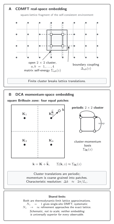
CDMFT and DCA retain different finite sets of nonlocal degrees of freedom while approximating an infinite lattice. The open real-space cluster resolves site and bond structure; the periodic DCA cluster resolves patch momenta with $\Delta k\sim2\pi/L_c$. The diagram is schematic and not to scale. Neither finite auxiliary cluster is the thermodynamic lattice.

The structured figure description records every object, relation, limit, and nonclaim without relying on the image.

Question	CDMFT	DCA
Cluster representation	open real-space cluster	periodic cluster and momentum patches
Finite-$N_c$ symmetry	lattice translations are broken	cluster translations are preserved; momenta are coarse-grained
Natural direct output	site-matrix correlators	patch-momentum correlators
Resolution scale	retained real-space separations and boundary-to-bulk ratio	patch diameter, typically $\Delta k\sim2\pi/L_c$
Characteristic drift	edge, cluster-shape, estimator, and periodization dependence	patch-shape, momentum-shell, and coarse-graining dependence
Exact-limit checks	$N_c=1$ gives single-site DMFT; appropriate compact sequences with $L_c\to\infty$ recover the lattice	the same limits, through a systematic refining patch sequence

To match Maier et al.’s large-cluster analysis, let $\boldsymbol\Gamma$ denote the cluster-to-medium hybridization kernel—the bath role carried by $\boldsymbol\Delta$ above—and use their frequency-inclusive trace

$$\overline\Gamma=\frac1{N_c}\operatorname{Tr}_{c,\omega}\boldsymbol\Gamma.$$

The trace runs over cluster labels and frequency; this is not the pointwise quantity $N_c^{-1}\operatorname{Tr}_c\boldsymbol\Gamma(z)$. For fixed dimension, short-ranged hopping, and regular compact cluster sequences with $N_c\sim L_c^d$, Maier et al. 2005, § II.D.5, printed p. 1042, eqs. (72)–(73) find

$$\overline\Gamma_{\mathrm{CDMFT}}=O(L_c^{-1}), \qquad \overline\Gamma_{\mathrm{DCA}}=O(L_c^{-2}).$$

These are asymptotic properties of the standard constructions, not universal error bars for every observable and not a theorem that DCA is always better at the same $N_c$. Observable convergence can be nonmonotonic and shape dependent, especially for exceptional small clusters.

Lattice reconstruction is a second approximation

Periodization is the nonunique reconstruction of a translationally invariant lattice quantity from finite-cluster data. CDMFT directly returns matrices on an open cluster, not a unique lattice spectrum. With the Fourier convention stated above, define

$$\mathcal P[X_c](\mathbf k,z) =\frac1{N_c}\sum_{ab} e^{-i\mathbf k\cdot(\mathbf r_a-\mathbf r_b)}X_{c,ab}(z).$$

Equivalently, $\mathcal P[X_c]=v_{\mathbf k}^\dagger X_c v_{\mathbf k}$ with $(v_{\mathbf k})_a=e^{i\mathbf k\cdot\mathbf r_a}/\sqrt{N_c}$. The three common choices make $\boldsymbol\Sigma_c$, the cluster cumulant $\mathbf M_c$, or the $\widetilde{\mathbf k}$-resolved lattice Green matrix translationally invariant. They agree in controlled limits but need not agree at finite $N_c$.

Self-energy periodization sets

$$\Sigma_\Sigma(\mathbf k,z)=\mathcal P[\boldsymbol\Sigma_c](\mathbf k,z), \qquad G_\Sigma(\mathbf k,z)= \frac1{z+\mu-\epsilon_{\mathbf k}-\Sigma_\Sigma(\mathbf k,z)}.$$

Cumulant periodization instead starts from

$$\mathbf M_c(z)=\left[(z+\mu)\mathbf1-\boldsymbol\Sigma_c(z)\right]^{-1},$$

and reconstructs

$$M(\mathbf k,z)=\mathcal P[\mathbf M_c](\mathbf k,z), \qquad G_M(\mathbf k,z)= \frac1{M(\mathbf k,z)^{-1}-\epsilon_{\mathbf k}}.$$

A Green-function reconstruction Fourier transforms the $\widetilde{\mathbf k}$-resolved lattice matrix

$$\mathbf G(\widetilde{\mathbf k},z) =\left[(z+\mu)\mathbf1-\mathbf t(\widetilde{\mathbf k}) -\boldsymbol\Sigma_c(z)\right]^{-1},$$

and then forms

$$G_G(\mathbf k,z)=\frac1{N_c}\sum_{ab} e^{-i\mathbf k\cdot(\mathbf r_a-\mathbf r_b)} G_{ab}(\widetilde{\mathbf k},z),$$

where $\widetilde{\mathbf k}$ is the reduced-zone representative of the full momentum $\mathbf k$. This is not merely the Fourier transform of the impurity matrix $\mathbf G_c$. These constructions and their strong-coupling differences are developed in Sakai et al. 2012, § II, printed pp. 035102-2–035102-3, eqs. (4)–(11), and Appendix A, printed pp. 035102-9–035102-10; the cumulant construction also appears in Stanescu and Kotliar 2006, printed pp. 125110-2–125110-3, eqs. (5)–(7).

Near a Mott self-energy pole, interpolating $\Sigma$ can be ill conditioned while the cumulant may be smoother; elsewhere that advantage need not hold. The different reconstructions can therefore move a gap edge or a putative zero surface. Report direct cluster observables first. For CDMFT, state whether a local estimator uses a central site, a boundary site, all sites, or selected bonds, and keep that estimator fixed along the cluster sequence. Compare at least two justified reconstructions before making a momentum-resolved claim.

For retarded functions, the quadratic-form identity gives

$$-\operatorname{Im}_H X_c^R(\omega)\succeq0 \quad\Longrightarrow\quad -\operatorname{Im}\mathcal P[X_c^R](\mathbf k,\omega)\ge0.$$

That useful sign check does not make nonlinear self-energy, cumulant, and Green-function reconstructions equivalent. In the standard CDMFT and DCA loops described here, a periodized or interpolated lattice output is postprocessing and is not fed back into a different fixed-point equation Maier et al. 2005, § II.C.3, printed p. 1039.

Two-particle response is a separate reconstruction

A one-particle spectrum does not supply a lattice susceptibility. A magnetic, charge, pairing, or nematic response requires measuring the connected cluster four-point function, extracting the irreducible vertex in a declared channel, and solving the corresponding lattice Bethe–Salpeter equation with the same CDMFT embedding or DCA coarse-graining. The frequency cutoff, cluster or patch indices, covariance, crossing relations, and applicable Ward identities must be checked independently.

Neither a periodized product of one-particle Green functions nor the auxiliary cluster susceptibility is automatically the lattice response. A one-particle momentum-selective suppression can motivate an ordering test, but it does not establish the broken symmetry or its thermodynamic transition.

A validity protocol for nonlocal claims

First converge the matrix fixed point and inspect imaginary-axis quantities. Define the Hermitian matrix imaginary part by

$$\operatorname{Im}_{H}\mathbf X =\frac{\mathbf X-\mathbf X^\dagger}{2i}.$$

For a retarded calculation, require both a causal bath and a causal solver output:

$$-\operatorname{Im}_{H}\boldsymbol\Delta^R(\omega)\succeq0, \qquad -\operatorname{Im}_{H}\boldsymbol\Sigma_c^R(\omega)\succeq0,$$

The solver must produce the self-energy sign, and the self-consistency map must preserve the bath sign. Given a causal input self-energy, the standard CDMFT map preserves bath causality Kotliar et al. 2001, printed pp. 186401-3–186401-4, eqs. (12)–(15); DCA has the corresponding causal construction Hettler et al. 2000, § IV.D and Appendix C, printed pp. 12744–12745 and 12754–12755. These statements do not certify an arbitrary approximate solver.

Also require

$$-\frac1\pi\operatorname{Im}_H\mathbf G_c^R(\omega)\succeq0, \qquad A(\mathbf k,\omega)=-\frac1\pi\operatorname{Im}G^R(\mathbf k,\omega)\ge0,$$

together with normalization, analyticity, and high-frequency moments such as $\lim_{|z|\to\infty}zG(\mathbf k,z)=1$. Positivity alone is not a complete validation.

A defensible nonlocal claim follows a staged protocol:

1. Declare the problem. Give $d$, $\epsilon_{\mathbf k}$, $U/t$, $\mu$ or $n$, $T/t$, boundary and cluster conventions, symmetry sector, solver, estimator, frequency grid, and target observable.
2. Converge the fixed point. Report $R_G$, $R_\Sigma$, observable drift, tail moments, initialization, mixing, and every coexisting branch. A small residual is necessary, not sufficient.
3. Separate solver error. For exact diagonalization, vary bath-site count, fit window and weights, and bath-fit tolerance. For CT-QMC, report average sign or phase, warmup, autocorrelation and binning, effective independent samples, and the full index-frequency covariance. Propagate resampled correlated data through matrix inversion, periodization, and continuation. The dedicated NRG and CT-QMC validity page develops these controls.
4. Vary the cluster approximation. Change $L_c$, $N_c$, shape, boundary convention, and point-group or momentum-shell bias; compare CDMFT and DCA when both address the same observable. Hold the local or bond estimator fixed. Near long correlation lengths, show the behavior with $L_c/\xi$ and cluster commensurability.
5. Separate reconstruction from continuation. Compare self-energy, cumulant, and Green-function periodizations on the imaginary axis first. Treat reconstruction spread as a systematic sensitivity bracket, not a Monte Carlo confidence interval. Only then vary continuation priors, grids, resolution, and synthetic-recovery tests.
6. Test phase claims in two stages. Hold the symmetry sector fixed while measuring cluster drift, then repeat every relevant competing sector. Two converged fixed points establish coexistence or metastability, not the stable phase. A first-order boundary requires a thermodynamically consistent grand-potential comparison; quote spinodals separately.

A four-site plaquette can establish short-range differentiation within that approximation. It cannot establish a thermodynamic phase boundary without drift data. Cluster size alone is not a convergence coordinate: two clusters with the same $N_c$ can have different $L_c$, symmetry, boundary weight, or commensurability. Long correlation lengths, stripes that fit one cluster but not another, and a sign change between reconstructions are characteristic stop conditions.

A worked momentum-selective test

A published two-dimensional benchmark makes the protocol concrete without turning its result into a universal phase claim. Sakai et al. studied the square-lattice dispersion

$$\epsilon_{\mathbf k}=-2t(\cos k_x+\cos k_y) -4t'\cos k_x\cos k_y$$

with $t'=-0.2t$, $U=8t$, $T=0.06t$, paramagnetic symmetry, fillings $n=0.99$, $0.97$, and $0.95$, and CDMFT clusters of $N_c=4,8,12,16$, including two distinct 12-site shapes Sakai et al. 2012, printed pp. 035102-1–035102-2 and Appendix B. Here the lowest fermionic Matsubara frequency is $\omega_0=\pi T\simeq0.19t$, which sets an important imaginary-axis energy-resolution scale. Their inability to push the largest cluster to lower temperature or larger hole doping because of the sign problem is part of the evidence boundary, not a footnote to discard.

Before analytic continuation, use the thermally broadened zero-energy proxy

$$\begin{aligned} G(\mathbf k,\beta/2) &=-\int_{-\infty}^{\infty} \frac{A(\mathbf k,\omega)}{2\cosh(\beta\omega/2)}\,\mathrm d\omega,\\ W(\mathbf k;\beta) &=-\frac\beta\pi G(\mathbf k,\beta/2). \end{aligned}$$

At finite $\beta$, $W$ is a normalized convolution of width $O(T)$, so $W(\mathbf k;\beta)\approx A(\mathbf k,0)$ only when $A$ is nearly constant across that window. If $A$ is continuous at $\omega=0$, then $W\to A(\mathbf k,0)$ as $\beta\to\infty$. It is not proof of a hard gap.

Sakai et al. plotted $-\beta G_M(\mathbf k,\beta/2)$ using cumulant periodization at $n=0.95$ for the main cluster sequence; their same-size shape comparison used the cumulant-periodized $\Sigma(\mathbf k,i\omega_0)$ rather than a full reconstruction-by-shape grid Sakai et al. 2012, § III.C, printed pp. 035102-6–035102-8, eq. (14) and Fig. 8(a), and Appendix B, Fig. 9. A new calculation following this protocol should compare nodal and antinodal $W$, direct cluster components, and any continued spectrum across the cluster sequence, both 12-site shapes, and at least self-energy and cumulant reconstructions. It should carry the CT-QMC covariance and sign limitations through the comparison. The article does not publish full covariance or average-sign data, so that part of the modern audit cannot be reconstructed from the paper alone.

The strongest conclusion is the one common to those tests: perhaps a stable low-energy momentum differentiation in the declared normal state, but not automatically a hard gap, a unique microscopic mechanism, or a thermodynamic pseudogap boundary. The successor pseudogap evidence page applies that distinction. The shared validity map and claim-validity table give the corresponding stop conditions and evidence ceiling.

Common pitfalls

Treating the auxiliary cluster as a finite lattice. CDMFT and DCA approximate an infinite lattice at every $N_c$. The relevant drift is with cluster correlation range, geometry, and resolution, not an ordinary physical-volume extrapolation.

Choosing the smoothest periodization. Smoothness is not correctness. Prefer direct cluster quantities, exact moments, causality, agreement among justified reconstructions, and stability along a controlled cluster sequence.

Calling one cluster size a sequence. Equal $N_c$ does not imply equal $L_c$, symmetry, boundary weight, or commensurability. A single plaquette is one approximation point.

Equating numerical convergence with physical validity. Small fixed-point residuals do not control bath discretization, Monte Carlo sign and covariance, analytic continuation, competing symmetry sectors, or missing long-range correlations.

Exercises

Single-site limit. Show that $N_c=1$ reduces either cluster construction to single-site DMFT.

Solution

With one cluster site, every bold quantity is a scalar. The CDMFT reduced-zone average becomes $G_{\mathrm{loc}}=N^{-1}\sum_{\mathbf k}[z+\mu-\epsilon_{\mathbf k}-\Sigma]^{-1}$. DCA has one patch containing the whole Brillouin zone and gives the same average. In both cases $\mathcal G_0^{-1}=G_{\mathrm{loc}}^{-1}+\Sigma$, exactly the single-site DMFT update.

DCA bath update. Starting from the DCA fixed-point equations, derive the displayed update for $\Delta_{\mathbf K}(z)$.

Solution

The cluster Dyson equation is $\Sigma_{\mathbf K}=\mathcal G_{0,\mathbf K}^{-1}-\overline G_{\mathbf K}^{-1}$. Substitute $\mathcal G_{0,\mathbf K}^{-1}=z+\mu-\bar\epsilon_{\mathbf K}-\Delta_{\mathbf K}$ and solve for the hybridization:

$$\Delta_{\mathbf K}=z+\mu-\bar\epsilon_{\mathbf K} -\Sigma_{\mathbf K}-\overline G_{\mathbf K}^{-1}.$$

Every term has units of energy. The update is patch dependent because $\bar\epsilon_{\mathbf K}$, $\Sigma_{\mathbf K}$, and $\overline G_{\mathbf K}$ are all patch dependent.

Periodization near a Mott pole. Why can self-energy and cumulant periodization disagree most strongly near a Mott gap?

Solution

A Mott gap can be associated with a self-energy pole. Fourier reconstructing a rapidly varying or divergent $\Sigma$ is ill conditioned, whereas $M=[z+\mu-\Sigma]^{-1}$ can remain smoother. That advantage is regime dependent, not a theorem. Their disagreement is observable reconstruction sensitivity that must be reported, not an uncertainty that can be hidden.

Local self-energy check. Let $\Sigma_{c,ab}(z)=\delta_{ab}\Sigma(z)$. Show that self-energy- and cumulant-style periodizations cannot create additional momentum dependence in the irreducible interaction correction.

Solution

The reconstruction gives

$$\mathcal P[\boldsymbol\Sigma_c](\mathbf k,z) =\frac1{N_c}\sum_a\Sigma(z)=\Sigma(z),$$

independent of $\mathbf k$. Likewise $\mathbf M_c=[z+\mu-\Sigma(z)]^{-1}\mathbf1$, so cumulant reconstruction gives $\Sigma_M=z+\mu-M^{-1}=\Sigma(z)$. The lattice Green function still varies with momentum through $\epsilon_{\mathbf k}$:

$$G(\mathbf k,z)= \frac1{z+\mu-\epsilon_{\mathbf k}-\Sigma(z)}.$$

Thus the periodizations add no momentum dependence to the interaction correction; they do not make the full propagator momentum independent.

Matrix causality. Let

$$-\operatorname{Im}_H\boldsymbol\Delta^R =\begin{pmatrix}a&b\\b^*&c\end{pmatrix}.$$

Find the conditions for this $2\times2$ Hermitian matrix to be positive semidefinite. Why are nonnegative diagonal entries insufficient? Then show that a direct Fourier quadratic form preserves the sign.

Solution

The principal-minor conditions are

$$a\ge0,\qquad c\ge0,\qquad ac\ge|b|^2.$$

Positive diagonal entries alone allow a negative eigenvalue when $|b|^2>ac$. If $H=-\operatorname{Im}_H\boldsymbol\Delta^R\succeq0$, then for the normalized Fourier vector $v_{\mathbf k}$,

$$-\operatorname{Im}\mathcal P[\boldsymbol\Delta^R] =v_{\mathbf k}^\dagger H v_{\mathbf k}\ge0.$$

This certifies the linear quadratic form, not every nonlinear reconstruction built from it.

Two-particle boundary. A periodized one-particle Green function has a strong antinodal suppression. Why does this not by itself establish an antiferromagnetic or pairing susceptibility divergence?

Solution

A susceptibility contains a two-particle vertex, not only a product of dressed one-particle propagators. One must measure the cluster four-point function, extract the irreducible vertex in the chosen channel, reconstruct the lattice bubble and vertex consistently, and solve the Bethe–Salpeter equation while controlling frequency cutoffs, covariance, cluster drift, and competing sectors. A one-particle suppression is compatible with several mechanisms and does not identify broken symmetry.

Evidence ceiling for a plaquette. A plaquette CDMFT calculation shows an antinodal suppression after self-energy periodization, but cumulant periodization moves the gap edge substantially and a second cluster shape is unconverged. What survives?

Solution

Only a plaquette- and reconstruction-dependent tendency toward momentum differentiation. The calculation has not established a thermodynamic pseudogap boundary. One should report the direct cluster and imaginary-axis quantities, reduce solver error, compare a controlled cluster sequence, and carry the reconstruction spread as a systematic sensitivity bracket rather than a statistical confidence interval.

References

• Matthias H. Hettler, A. N. Tahvildar-Zadeh, Mark Jarrell, Thomas Pruschke, and H. R. Krishnamurthy, “Nonlocal Dynamical Correlations of Strongly Interacting Electron Systems,” Physical Review B 58 (1998) R7475–R7479, doi:10.1103/PhysRevB.58.R7475.
• Matthias H. Hettler, M. Mukherjee, Mark Jarrell, and H. R. Krishnamurthy, “Dynamical Cluster Approximation: Nonlocal Dynamics of Correlated Electron Systems,” Physical Review B 61 (2000) 12739–12756, doi:10.1103/PhysRevB.61.12739.
• Gabriel Kotliar, Sergej Y. Savrasov, Gunnar Pálsson, and Giulio Biroli, “Cellular Dynamical Mean Field Approach to Strongly Correlated Systems,” Physical Review Letters 87 (2001) 186401, doi:10.1103/PhysRevLett.87.186401.
• Thomas Maier, Mark Jarrell, Thomas Pruschke, and Matthias H. Hettler, “Quantum Cluster Theories,” Reviews of Modern Physics 77 (2005) 1027–1080, §§ II–IV, doi:10.1103/RevModPhys.77.1027.
• Shiro Sakai, Giorgio Sangiovanni, Marcello Civelli, Yukitoshi Motome, Karsten Held, and Masatoshi Imada, “Cluster-Size Dependence in Cellular Dynamical Mean-Field Theory,” Physical Review B 85 (2012) 035102, doi:10.1103/PhysRevB.85.035102.
• Tudor D. Stanescu and Gabriel Kotliar, “Fermi Arcs and Hidden Zeros of the Green Function in the Pseudogap State,” Physical Review B 74 (2006) 125110, doi:10.1103/PhysRevB.74.125110.