Sign-Free Quantum Monte Carlo and Hubbard-Phase Inference

Sign-free auxiliary-field quantum Monte Carlo is a symmetry theorem followed by a convergence protocol. For the half-filled repulsive Hubbard model on a bipartite hopping graph, and for the attractive model with identical real spin-sector one-body matrices, every auxiliary-field configuration can carry a nonnegative weight. Antiunitary symmetries extend this statement to some conjugate complex sectors. Sign freedom removes exponential sign cancellations; it does not remove equilibration, autocorrelation, matrix-conditioning, time-step, projection, finite-size, estimator, or interpretation errors.

Required background. Use Hubbard symmetries to identify the particle–hole-symmetric point, Markov-chain sampling to interpret correlated samples, and sign-problem anatomy to distinguish a configuration sign from an average sign. Helpful background. Covariance and resampling supplies the error analysis used below.

From the Hubbard interaction to a determinant

Write the shifted single-band Hubbard Hamiltonian as

$$H=\widehat K +U\sum_i\left(n_{i\uparrow}-\frac12\right) \left(n_{i\downarrow}-\frac12\right),$$

where

$$\widehat K =\sum_{ij\sigma}c_{i\sigma}^\dagger k_{ij}c_{j\sigma}, \qquad k_{ij}=-t_{ij}-\widetilde\mu\,\delta_{ij}.$$

The shifted chemical potential is $\widetilde\mu=0$ at half filling on the particle–hole-symmetric bipartite model. In the unshifted convention $U n_{i\uparrow}n_{i\downarrow}-\mu(n_{i\uparrow}+n_{i\downarrow})$, the same point is $\mu=U/2$.

For inverse temperature $\beta=L_\tau\Delta\tau$, a symmetric time slice obeys

$$e^{-\Delta\tau(\widehat K+\widehat V)} =e^{-\Delta\tau\widehat K/2} e^{-\Delta\tau\widehat V} e^{-\Delta\tau\widehat K/2} +O(\Delta\tau^3).$$

At fixed finite $\beta$ and lattice, the accumulated leading error in a regular observable is quadratic:

$$\langle O\rangle_{\Delta\tau} =\langle O\rangle_0+c_2\Delta\tau^2+O(\Delta\tau^4).$$

The coefficient depends on the system, observable, size, temperature, and commutators. The formal breakup predicts a fit variable; it does not replace a $\Delta\tau\to0$ study.

For $U>0$, Hirsch’s discrete spin-channel identity is

$$e^{-\Delta\tau U(n_\uparrow-1/2)(n_\downarrow-1/2)} =\frac{e^{-\Delta\tau U/4}}{2} \sum_{s=\pm1}e^{\lambda s(n_\uparrow-n_\downarrow)}, \qquad \cosh\lambda=e^{\Delta\tau U/2}.$$

For a fixed Ising-field history $s_{i\ell}=\pm1$, define the diagonal matrices

$$[v_{\ell\uparrow}]_{ij}=+\lambda s_{i\ell}\delta_{ij}, \qquad [v_{\ell\downarrow}]_{ij}=-\lambda s_{i\ell}\delta_{ij},$$

and the one-particle slice and full propagators

$$\begin{aligned} B_{\ell\sigma} &=e^{-\Delta\tau k/2}e^{v_{\ell\sigma}}e^{-\Delta\tau k/2},\\ \mathcal B_\sigma(\beta,0) &=B_{L_\tau\sigma}\cdots B_{2\sigma}B_{1\sigma}. \end{aligned}$$

The grand-canonical fermion trace produces the fermion matrix

$$M_\sigma[s]=I+\mathcal B_\sigma(\beta,0),$$

not $\mathcal B_\sigma$ itself. The discretized partition function is

$$Z_{\Delta\tau} =\sum_{\{s\}}W[s], \qquad W[s]=p_{\rm HS}[s]\det M_\uparrow[s]\det M_\downarrow[s],$$

where $p_{\rm HS}[s]>0$ contains every scalar factor from the auxiliary-field identity. The many-fermion trace-to-determinant reduction and symmetric sliced evolution are given in Blankenbecler, Scalapino, and Sugar 1981, §§ II–III, printed pp. 2279–2282, eqs. (24)–(43). The discrete fields and explicit fermion trace are given in Hirsch 1983, printed pp. 4059–4060, eqs. (10) and (14)–(16), with the 1984 correction to eq. (10b).

Once $s$ is fixed, the interacting problem has become quadratic: the fermionic Fock-space trace is the determinant above, and equal-time observables follow from a one-particle Green matrix. At the time boundary implicit in the ordering of $\mathcal B_\sigma$ above, use

$$G^\sigma_{ij}[s] =\langle c_{i\sigma}c_{j\sigma}^\dagger\rangle_s, \qquad G^\sigma[s]=M_\sigma^{-1}[s].$$

At an arbitrary slice $\ell$, cyclically order the propagators around that slice:

$$G^\sigma_\ell[s] =\left[ I+B_{\ell\sigma}\cdots B_{1\sigma} B_{L_\tau\sigma}\cdots B_{(\ell+1)\sigma} \right]^{-1}.$$

Then $n_{i\sigma}[s]=1-G^\sigma_{ii}[s]$, and Wick’s theorem gives

$$\langle n_{i\sigma}n_{j\sigma}\rangle_s =n_{i\sigma}[s]n_{j\sigma}[s] +\bigl(\delta_{ij}-G^\sigma_{ji}[s]\bigr)G^\sigma_{ij}[s].$$

Opposite-spin contractions factorize at fixed $s$ before the auxiliary-field average. This is the bridge from determinant sampling to magnetic, density, and pairing estimators.

Two standard nonnegative domains

Repulsive model at half filling

Let $D_{ij}=\eta_i\delta_{ij}$ with $\eta_i=+1$ on sublattice $A$ and $-1$ on sublattice $B$. The required finite-matrix condition is

$$Dk^{\mathsf T}D=-k.$$

For real symmetric hopping this reduces to $DkD=-k$. It requires $\widetilde\mu=0$ and a boundary graph containing only opposite-sublattice hopping; an odd periodic cycle or same-sublattice hopping can invalidate it even when the infinite bulk lattice looks bipartite.

Apply the partial particle–hole transformation

$$c_{i\downarrow}\longmapsto \eta_i c_{i\downarrow}^\dagger.$$

With the uncentered one-body matrices defined above, a down-spin field factor transforms as

$$e^{-\lambda s n_\downarrow} \longmapsto e^{-\lambda s}e^{+\lambda s n_h}.$$

Consequently,

$$\det M_\downarrow[s] =e^{-\lambda\sum_{i\ell}s_{i\ell}} \det M_\uparrow[s],$$

and the configuration weight is

$$W[s] =p_{\rm HS}[s] e^{-\lambda\sum_{i\ell}s_{i\ell}} \bigl(\det M_\uparrow[s]\bigr)^2\ge0.$$

The exponential is positive and may be absorbed into the sampling measure. It may not be dropped from an equality between the two bare determinants. Hirsch derives this field-dependent proportionality in Hirsch 1985, § III, printed pp. 4406–4407, eqs. (3.9)–(3.12).

Doping away from $\widetilde\mu=0$, adding real same-sublattice hopping, or choosing a nonbipartite finite cluster removes this proof. That statement identifies the boundary of this sufficient theorem; it does not classify every possible sign-free Hamiltonian.

Attractive model with identical spin sectors

For $U=-|U|<0$, use the charge channel

$$e^{+\Delta\tau |U|(n_\uparrow-1/2)(n_\downarrow-1/2)} =\frac{e^{-\Delta\tau |U|/4}}{2} \sum_{s=\pm1}e^{\lambda s(n_\uparrow+n_\downarrow-1)}, \qquad \cosh\lambda=e^{\Delta\tau |U|/2}.$$

This is the corrected attractive charge-channel identity in Hirsch 1983, printed p. 4059, eq. (10b), with its scalar factor and sign corrected in the Hirsch 1984 erratum, printed p. 4159.

Equivalently, each field term is $e^{-\lambda s}e^{\lambda s n_\uparrow}e^{\lambda s n_\downarrow}$. Absorb the positive scalar $e^{-\lambda s}$ into $p_{\rm HS}$ and set

$$[v_{\ell\uparrow}]_{ij} =[v_{\ell\downarrow}]_{ij} =\lambda s_{i\ell}\delta_{ij}.$$

If the up and down sectors have identical real one-body matrices—real spin-independent hopping, a common chemical potential, and real-preserving boundary conditions—then

$$M_\uparrow[s]=M_\downarrow[s]=M[s], \qquad \det M[s]\in\mathbb R,$$

so $W[s]=p_{\rm HS}[s](\det M[s])^2\ge0$. A common chemical potential at arbitrary filling and real frustrating hopping preserve this equality; bipartiteness is not required. Equal mean populations alone are insufficient—the two one-body matrices must agree configuration by configuration. A generic boundary twist complexifies the hopping and is not covered by this real-square proof. If instead a protecting antiunitary symmetry gives $M_\downarrow=M_\uparrow^*$, the product is $|\det M_\uparrow|^2\ge0$. Spin-dependent chemical potentials or hopping remove the simple equality, though another symmetry may still protect a particular model Batrouni and de Forcrand 1993, printed pp. 589–590, eqs. (2)–(6).

A broader antiunitary criterion

The two examples above factor into spin determinants, but factorization is not the general theorem. Suppose an antiunitary operator $\mathcal T$ leaves every auxiliary-field one-body slice invariant and satisfies $\mathcal T^2=-1$. Eigenvalues of the full fermion matrix then occur in complex-conjugate pairs, while real eigenvalues are Kramers-degenerate. Therefore

$$\det M=\prod_a |\lambda_a|^2\ge0.$$

This is a sufficient condition, not a necessary classification, and it need not be expressible as two spin-block determinants forming a modulus square Wu and Zhang 2005, § III, printed pp. 155115-3–155115-4, eqs. (13)–(17).

Thermal and projector AFQMC are different ensembles

Finite-temperature determinant QMC takes a trace and therefore contains $\det[I+\mathcal B_\sigma(\beta,0)]$. Ground-state projector AFQMC starts from a trial Slater determinant $|\Psi_T\rangle$ and instead evaluates

$$\langle O\rangle_0 =\lim_{\Theta\to\infty} \frac{ \langle\Psi_T|e^{-\Theta H}Oe^{-\Theta H}|\Psi_T\rangle }{ \langle\Psi_T|e^{-2\Theta H}|\Psi_T\rangle }.$$

If $P_\sigma$ is the matrix of occupied trial orbitals, the projector weight has the form

$$W_{\rm P}[s] =p_{\rm HS}[s]\prod_\sigma \det\!\left[ P_\sigma^\dagger \mathcal B_\sigma(2\Theta,0) P_\sigma \right].$$

There is no $I+\mathcal B$ because the determinant is an overlap in a selected particle-number sector, not a grand-canonical trace. Three conditions matter:

• The trial state must have nonzero overlap with the ground state in the target particle-number and symmetry sector. Projection cannot repair an exactly wrong sector.
• A generic excited-state contamination falls as $e^{-\Theta\Delta_L}$, where $\Delta_L$ is the relevant finite-size gap. Near a quantum critical point $\Delta_L\sim L^{-z}$, so either hold $\Theta/L^z$ fixed for a critical aspect-ratio study or demonstrate ground-state convergence separately.
• A sign-free projector weight requires trial determinants compatible with the protecting particle–hole or antiunitary symmetry. An arbitrary trial determinant does not inherit positivity automatically.

Inside an unconstrained sign-free formulation, the trial state controls overlap, convergence rate, and variance, but not the $\Theta\to\infty$ answer for a unique ground state in the target sector—or after the desired vector has been fixed inside a degenerate ground-state subspace. With an exactly degenerate ground manifold, projection retains the trial state’s components in that manifold, so observables can depend on those components. A constrained-path or phaseless approximation used outside the proved domain introduces an additional trial-state bias. The projection and overlap requirements originate with Sugiyama and Koonin 1986, printed p. 2, eq. (1), and §§ II.1–II.2, printed pp. 2–5; a Hubbard implementation appears in White et al. 1989, § II.B, printed pp. 509–511, eqs. (21)–(28).

Long products of $B$ matrices become severely ill-conditioned at low temperature or long projection length. QR, UDT, or SVD stabilization, periodic Green-function recomputation, and tolerance or precision checks are part of the definition of a trustworthy result, not optional performance details.

A finite-size estimator for magnetic order

Let $N$ be the number of sites, $\mathbf S_i=\tfrac12c_i^\dagger\boldsymbol\sigma c_i$, and $\mathbf Q$ the ordering wavevector. Define the equal-time structure factor

$$S(\mathbf Q) =\frac1N\sum_{ij} e^{i\mathbf Q\cdot(\mathbf r_i-\mathbf r_j)} \langle\mathbf S_i\cdot\mathbf S_j\rangle, \qquad m_L^2=\frac{S(\mathbf Q)}{N}.$$

If only $S^{zz}$ is measured and the state is SU(2)-symmetric, use $m_L^2=3S^{zz}(\mathbf Q)/N$. Do not interchange the equal-time structure factor with the time-integrated susceptibility; their scaling dimensions differ.

For a periodic box of linear size $L$ and unit lattice spacing, choose the smallest momentum increment $\delta\mathbf q=(2\pi/L)\hat{\mathbf e}$ in a declared direction and define

$$R_L =1-\frac{S(\mathbf Q+\delta\mathbf q)}{S(\mathbf Q)}.$$

An average over symmetry-related nearest momenta is often less direction-sensitive. The corresponding second-moment length is

$$\xi_L =\frac{1}{2\sin(|\delta q|/2)} \sqrt{ \frac{S(\mathbf Q)}{S(\mathbf Q+\delta\mathbf q)}-1 }.$$

Thus $R_L=y_L^2/(1+y_L^2)$ with $y_L=2\sin(|\delta q|/2)\xi_L$. In a short-range disordered phase $R_L\to0$; in an ordered phase the Bragg peak dominates and $R_L\to1$; at a conventional continuous transition it approaches a nontrivial scaling value. Chen et al. use this momentum-space ratio and its crossings in Chen et al. 2019, printed p. 077601-2, Fig. 2(a), with the scaling collapse in Fig. 3.

For a conventional zero-temperature critical point,

$$R_L(g,\beta) =F_R\!\left((g-g_c)L^{1/\nu},\frac{\beta}{L^z}\right) +L^{-\omega}G_R+\cdots,$$

and

$$m_L^2 =L^{-(d+z-2+\eta)} F_m\!\left((g-g_c)L^{1/\nu},\frac{\beta}{L^z}\right) +\cdots.$$

At a finite-temperature classical transition, omit $z$ and use $m_L^2\sim L^{-(d-2+\eta)}$ at criticality. For a fixed size ratio $s>1$, expand

$$R_L(g)=F\!\left((g-g_c)L^{1/\nu}\right) +L^{-\omega}G\!\left((g-g_c)L^{1/\nu}\right)+\cdots.$$

If $F'(0)$ and the leading correction amplitude are nonzero, the pairwise crossing drifts as

$$g^\times_{L,sL}-g_c =\frac{G(0)(1-s^{-\omega})} {F'(0)(s^{1/\nu}-1)} L^{-(1/\nu+\omega)}+\cdots.$$

The figure separates a finite size-pair crossing from the conditional thermodynamic intercept. Its correction coordinate is $x_L=L^{-(1/\nu+\omega)}$; inspect the distinct crossing locations before reading the extrapolation.

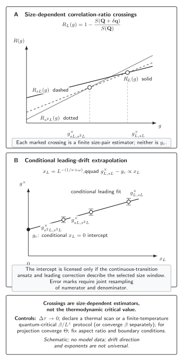
Schematic correlation-ratio analysis for an ordinary continuous transition. Successive sizes cross at distinct pair estimates; $g_c$ follows only from a declared correction-to-scaling fit with joint numerator–denominator covariance and independent control of time step, thermal-transition or finite-temperature quantum-critical protocol, projection length, aspect ratio, and boundaries. Curve shapes, error-mark sizes, drift direction, and exponents are illustrative, not universal, and no model data are shown.

The structured figure description records every curve, relation, assumption, limit, and nonclaim without relying on the image. The displayed power law is inappropriate for a first-order, Berezinskii–Kosterlitz–Thouless, multicritical, strongly anisotropic, or dangerously irrelevant scaling problem unless a separate derivation licenses it.

For uncertainty propagation, let $A=S(\mathbf Q+\delta\mathbf q)$ and $B=S(\mathbf Q)$. To first order,

$$\operatorname{Var}(R_L) \simeq \frac{\operatorname{Var}(A)}{B^2} +\frac{A^2\operatorname{Var}(B)}{B^4} -\frac{2A\operatorname{Cov}(A,B)}{B^3}.$$

Because $A$ and $B$ are measured on the same configurations, their covariance is compulsory. Recompute the ratio, crossings, and final fit inside a joint blocked jackknife or bootstrap rather than resampling raw autocorrelated measurements as if they were independent. Separate simulations at different $L$ normally have zero sampling cross-covariance; cross-size covariance exists only when common random numbers, disorder samples, reweighting, or shared calibration actually couples them. Covariance changes uncertainty and finite-sample bias—it is not a physical source of scaling drift.

Worked inference: the three-dimensional half-filled model

Staudt, Dzierzawa, and Muramatsu studied the repulsive Hubbard model at half filling on periodic simple-cubic $L\times L\times L$ lattices with finite-temperature grand-canonical determinant QMC. At $U/t=6$ they used $L=4,6,8,10$, set $t=1$, chose $\Delta\tau^2tU=0.1$ after time-step checks, and grouped between $100000$ measurement sweeps at $L=4$ and $2000$ at $L=10$ into 20 blocks Staudt, Dzierzawa, and Muramatsu 2000, § 2, printed p. 412.

Their magnetic convention was

$$S_{\rm H}(\mathbf Q) =\frac1{L^3}\sum_{ij} e^{i\mathbf Q\cdot(\mathbf R_i-\mathbf R_j)} \left\langle (n_{i\uparrow}-n_{i\downarrow}) (n_{j\uparrow}-n_{j\downarrow}) \right\rangle, \qquad \mathbf Q=(\pi,\pi,\pi),$$

with

$$\frac{S_{\rm H}(\mathbf Q)}{L^3}=m^2+f(L).$$

Since $n_{i\uparrow}-n_{i\downarrow}=2S_i^z$, SU(2) symmetry gives $S_{\rm H}=4S^{zz}=\tfrac43S$ in the rotationally invariant convention used earlier. Their extrapolated $m^2$ is therefore $\tfrac43m_L^2$ in that convention. The zero-versus-nonzero intercept is unchanged, but the quoted magnetization normalization is not numerically interchangeable.

They fitted the finite-size specific-heat peak locations empirically as $T_{\max}(L)=T_N+a/L$ and obtained $T_N/t=0.31\pm0.01$. That $1/L$ peak shift was their interpolation ansatz, not a universality-derived replacement for the general shift $L^{-1/\nu}$. For the independent magnetic check they fitted $f(L)\propto L^{-\lambda}$ with $\lambda$ allowed to float: the extrapolated intercept was nonzero at $T/t=0.30$ and consistent with zero at $0.36$ and $0.40$, and they omitted smaller sizes to test fit-range stability Staudt, Dzierzawa, and Muramatsu 2000, printed p. 413, eqs. (2)–(3) and Figs. 2–3.

This is a useful reconstruction of inference logic, not a new precision determination. The candidate transition from a thermodynamic feature was checked against the order parameter, and the finite-size conclusion was tested against fit range. The article does not publish integrated autocorrelation times, the covariance of the derived observables, raw blocked data, or a modern multi-$\Delta\tau$ joint extrapolation. The strongest reproducible statement is therefore that its specified finite-size analysis supports a Néel transition near the quoted temperature for that lattice Hamiltonian—not that every present-day systematic has been reconstructed.

Dimension changes the conclusion. A two-dimensional short-range SU(2)-symmetric Hubbard model cannot have finite-temperature antiferromagnetic long-range order. Growth of $S(\mathbf Q)$ or an apparent crossing at finite $\beta$ can mark $\xi\sim L$ in the renormalized-classical regime; it supports a correlation-length crossover or a controlled $T\to0$ inference, not $T_N>0$ Walker and Ruijgrok 1968, printed pp. 513–515.

Controls that license the conclusion

The simulation claim should survive these gates in this order:

1. Algebraic domain. Check the finite matrix, boundary conditions, twists, chemical potentials, and trial determinants against the actual positivity theorem. Test the configuration sign numerically as a diagnostic, not as a substitute for the proof.
2. Equilibration and autocorrelation. Remove warmup, estimate the slowest relevant integrated autocorrelation time, use blocks much longer than that time, report an effective sample size, and compare independent chains. Blocking and nonlinear derived-observable analysis are developed in Flyvbjerg and Petersen 1989, §§ II–IV, printed pp. 461–464, eqs. (20)–(27) and Wolff 2004, §§ 1 and 3.1, eqs. (31)–(39).
3. Stable arithmetic. Stabilize long matrix products, periodically recompute Green functions, and vary the factorization interval, tolerance, and precision. A nonnegative measure can still have determinant-zero singularities or infinite-variance estimators, so inspect tails and required moments Shi and Zhang 2016, §§ II–IV.
4. Time step and state preparation. Use several $\Delta\tau$ values to test the expected quadratic approach. Separately vary $\beta$ or $\Theta$ and the trial state; test cross-terms when projection, size, and time-step errors are comparable.
5. Covariance and finite size. Jointly resample every same-ensemble derived observable, keep shape and boundary conditions fixed, vary the minimum accepted size, and compare justified correction ansätze. Stop if the inferred limit depends materially on the fit window or on an unproved universality class.
6. Competing interpretations. Measure the relevant order parameters, stiffnesses, gaps, or correlation lengths instead of identifying a phase from the absence of one conventional order. The neighboring competing-orders page develops this comparison.
7. Continuation only when needed. Equal-time $S(\mathbf Q)$ and $R_L$ need no analytic continuation. A real-frequency claim must disclose the kernel, full imaginary-time covariance, default model or regularizer, sum rules, synthetic-resolution tests, and stability window; otherwise report only the imaginary-time observable Gubernatis et al. 1991, §§ II–III, printed pp. 6012–6020.

The general QMC phase-inference page owns the reusable sampling and scaling workflow. The chapter’s shared validity map and claim-validity table place sign-free QMC beside Hamiltonian reduction, DMFT, cluster methods, and competing-mechanism tests.

Evidence ceiling

At fixed finite lattice, $\beta$ or $\Theta$, $\Delta\tau$, boundary conditions, and estimator definition, equilibrated and numerically stable sampling of a proved nonnegative auxiliary-field measure is asymptotically exact for that regulated problem, provided the required moments exist. A physical phase claim additionally needs controlled time-step, thermal or projection, thermodynamic, covariance, and inference limits.

Sign freedom does not establish ergodicity, equilibration, stable arithmetic, finite variance, absence of nonlinear-estimator bias, or absence of constrained-path bias. It does not prove that the lattice model describes a material. Pairing enhancement is not by itself a superconducting transition, and failure to find one order does not identify the alternative phase.

Common pitfalls

Writing a bare determinant square for the repulsive shifted convention. The down determinant differs by a positive field-dependent exponential. Absorb that factor into the measure only after writing the correct equality.

Using an arbitrary trial state in projector QMC. Nonzero ground-state overlap and compatibility with the protecting symmetry are separate requirements. A long projection cannot recover a state in an exactly absent sector.

Calling one crossing the critical point. A crossing is a size-pair estimator. The thermodynamic value requires a stable, justified drift analysis and independent control of time-step and thermal or projector geometry.

Treating covariance as a scaling correction. Covariance controls the uncertainty of ratios and fits. Irrelevant operators, finite temperature or projection, Trotter error, geometry, and a poor scaling ansatz generate physical drift.

Exercises

For one orbital, one time slice, and $k=0$, show directly why the repulsive determinants in the displayed convention are not equal even though their product can enter a nonnegative weight.

Solution

For field $s=\pm1$,

$$M_\uparrow=1+e^{\lambda s}, \qquad M_\downarrow=1+e^{-\lambda s} =e^{-\lambda s}(1+e^{\lambda s}).$$

Thus $\det M_\downarrow=e^{-\lambda s}\det M_\uparrow$, not $\det M_\downarrow=\det M_\uparrow$. The factor is strictly positive, so

$$\det M_\uparrow\det M_\downarrow =e^{-\lambda s}(1+e^{\lambda s})^2\ge0.$$

The full lattice proof applies the same scalar factor at every site and slice after the bipartite particle–hole transformation.

For the attractive Hubbard model, explain why a common chemical-potential change preserves the determinant square while a spin-dependent change generally does not. State the additional reality condition.

Solution

The charge-channel auxiliary field is identical for both spins. A common chemical potential, hopping matrix, and boundary twist therefore give $M_\uparrow[s]=M_\downarrow[s]$ for every field configuration. With real one-body matrices, $\det M\in\mathbb R$, so the product is $(\det M)^2\ge0$ at any filling. A spin-dependent chemical potential makes the two matrices unequal and removes this proof. In a fixed-number projector calculation, a chemical potential is only a sector-dependent constant; the trial determinants and the remaining one-body terms must still satisfy the protecting relation.

Contrast the thermal determinant $\det[I+\mathcal B_\sigma]$ with the projector determinant $\det[P_\sigma^\dagger\mathcal B_\sigma P_\sigma]$. What happens if $|\Psi_T\rangle$ has zero overlap with the desired ground state?

Solution

The thermal determinant comes from tracing over the spin-$\sigma$ Fock space, which produces $I+\mathcal B_\sigma$. The projector determinant is the overlap of an evolved occupied-orbital subspace with the trial subspace, so it contains $P_\sigma^\dagger\mathcal B_\sigma P_\sigma$ and no identity term. Expanding $|\Psi_T\rangle=\sum_n a_n|n\rangle$ shows that projection multiplies each component by $e^{-\Theta E_n}$. If the target ground-state coefficient is exactly $a_0=0$, no projection length can create it; the calculation converges within the sector that actually has overlap.

Let $R=1-A/B$, where $A$ and $B$ are measured on the same Markov chain. Derive the leading covariance formula and explain how to estimate the uncertainty without pretending the samples are independent.

Solution

The gradient is $\partial R/\partial A=-1/B$ and $\partial R/\partial B=A/B^2$. The delta method gives

$$\operatorname{Var}(R) \simeq \frac{\operatorname{Var}(A)}{B^2} +\frac{A^2\operatorname{Var}(B)}{B^4} -\frac{2A\operatorname{Cov}(A,B)}{B^3}.$$

Choose blocks long compared with the slowest relevant autocorrelation time, then delete or resample whole blocks and recompute $A$, $B$, $R$, the crossing, and the final fit inside every jackknife or bootstrap replica. This retains both serial correlation and the same-configuration covariance. Independently generated lattice sizes do not acquire sampling covariance merely because they enter one fit.

Assume, as a heuristic rather than an exact interacting critical line shape, that

$$\frac{S(\mathbf Q+\mathbf q)}{S(\mathbf Q)} \simeq\frac{1}{1+\xi_L^2\mathbf q^2}.$$

For a periodic unit-lattice-spacing box, express $R_L$ using $\delta q=2\pi/L$. Explain its disordered and scale-invariant limits, and why a finite-temperature crossing in the two-dimensional SU(2)-symmetric Hubbard model is not evidence for a Néel transition.

Solution

Substitution gives

$$R_L\simeq \frac{\xi_L^2(2\pi/L)^2} {1+\xi_L^2(2\pi/L)^2}.$$

If $\xi_L\to\xi<\infty$, then $R_L=O(L^{-2})\to0$. If $\xi_L/L$ approaches a nonzero scaling function, $R_L$ approaches a size-independent value. This assumed Lorentzian is pedagogical; an interacting critical point can have an anomalous line shape. In two dimensions with short-range interactions and unbroken SU(2) symmetry, finite-temperature magnetic long-range order is forbidden. An apparent crossing can signal $\xi\sim L$ and strong renormalized-classical correlations, but only a controlled $T\to0$ or ground-state analysis can support antiferromagnetic order.

References

• Ghassan G. Batrouni and Philippe de Forcrand, “Fermion Sign Problem: Decoupling Transformation and Simulation Algorithm,” Physical Review B 48 (1993) 589–592, doi:10.1103/PhysRevB.48.589.
• Richard Blankenbecler, Douglas J. Scalapino, and Robert L. Sugar, “Monte Carlo Calculations of Coupled Boson–Fermion Systems. I,” Physical Review D 24 (1981) 2278–2286, doi:10.1103/PhysRevD.24.2278.
• Chuang Chen, Xiao Yan Xu, Zi Yang Meng, and Martin Hohenadler, “Charge-Density-Wave Transitions of Dirac Fermions Coupled to Phonons,” Physical Review Letters 122 (2019) 077601, doi:10.1103/PhysRevLett.122.077601.
• Henrik Flyvbjerg and H. G. Petersen, “Error Estimates on Averages of Correlated Data,” Journal of Chemical Physics 91 (1989) 461–466, doi:10.1063/1.457480.
• James E. Gubernatis, Mark Jarrell, R. N. Silver, and D. S. Sivia, “Quantum Monte Carlo Simulations and Maximum Entropy: Dynamics from Imaginary-Time Data,” Physical Review B 44 (1991) 6011–6029, doi:10.1103/PhysRevB.44.6011.
• Jorge E. Hirsch, “Discrete Hubbard–Stratonovich Transformation for Fermion Lattice Models,” Physical Review B 28 (1983) 4059(R)–4061, with erratum Physical Review B 29 (1984) 4159, doi:10.1103/PhysRevB.28.4059, erratum: doi:10.1103/PhysRevB.29.4159.
• Jorge E. Hirsch, “Two-Dimensional Hubbard Model: Numerical Simulation Study,” Physical Review B 31 (1985) 4403–4419, doi:10.1103/PhysRevB.31.4403.
• Hao Shi and Shiwei Zhang, “Infinite Variance in Fermion Quantum Monte Carlo Calculations,” Physical Review E 93 (2016) 033303, doi:10.1103/PhysRevE.93.033303.
• R. Staudt, M. Dzierzawa, and A. Muramatsu, “Phase Diagram of the Three-Dimensional Hubbard Model at Half Filling,” European Physical Journal B 17 (2000) 411–415, doi:10.1007/s100510070120, Open PDF.
• G. Sugiyama and Steven E. Koonin, “Auxiliary Field Monte-Carlo for Quantum Many-Body Ground States,” Annals of Physics 168 (1986) 1–26, doi:10.1016/0003-4916(86)90107-7.
• M. B. Walker and Th. W. Ruijgrok, “Absence of Magnetic Ordering in One and Two Dimensions in a Many-Band Model for Interacting Electrons in a Metal,” Physical Review 171 (1968) 513–515, doi:10.1103/PhysRev.171.513.
• Steven R. White, Douglas J. Scalapino, Robert L. Sugar, E. Y. Loh Jr., James E. Gubernatis, and Richard T. Scalettar, “Numerical Study of the Two-Dimensional Hubbard Model,” Physical Review B 40 (1989) 506–516, doi:10.1103/PhysRevB.40.506.
• Ulli Wolff, “Monte Carlo Errors with Less Errors,” Computer Physics Communications 156 (2004) 143–153, with erratum 176 (2007) 383, doi:10.1016/S0010-4655(03)00467-3, erratum: doi:10.1016/j.cpc.2006.12.001.
• Congjun Wu and Shou-Cheng Zhang, “Sufficient Condition for Absence of the Sign Problem in the Fermionic Quantum Monte Carlo Algorithm,” Physical Review B 71 (2005) 155115, doi:10.1103/PhysRevB.71.155115.