Bogoliubov–de Gennes Theory in Inhomogeneous Systems

Bogoliubov–de Gennes (BdG) theory turns a specified pairing saddle into a spatial quasiparticle problem. Once the one-body operator, pair field, regulator, ensemble, gauge, and boundary conditions are fixed, the method produces normalized particle–hole wavefunctions and electron observables such as the local density of states. It can also update the pair field self-consistently. The result is still a mean-field result: a converged subgap eigenvalue is not automatically a stable thermodynamic state, an open-system resonance, a topological mode, or a many-body addition energy.

Required background. Nambu–Gor’kov propagators fixes the reduced spin-singlet basis, anomalous sign, gauge transformation, and particle–hole counting rule.

Helpful background. Basis construction and symmetry sectors supplies finite-dimensional regulator and residual checks.

From a Nambu kernel to a spatial operator

Consider a balanced, even-parity spin-singlet saddle in the reduced basis

$$\Psi(\mathbf r) =\begin{pmatrix} \psi_\uparrow(\mathbf r)\\ \psi_\downarrow^\dagger(\mathbf r) \end{pmatrix}.$$

Let $q$ be the signed charge in the covariant momentum; for an electron, $q=-\lvert e\rvert$. Define

$$K =\frac{[-i\boldsymbol\nabla-q\mathbf A(\mathbf r)]^2}{2m} +V(\mathbf r)-\mu .$$

For local singlet pairing, the closed-system BdG operator is

$$H_{\mathrm{BdG}} =\begin{pmatrix} K&\Delta(\mathbf r)\\ \Delta^\ast(\mathbf r)&-K^\ast \end{pmatrix}, \qquad H_{\mathrm{BdG}}\Psi_n=E_n\Psi_n, \qquad \Psi_n=\begin{pmatrix}u_n\\v_n\end{pmatrix}.$$

This is an operator equation, not a pointwise $2\times2$ matrix: $K$ contains derivatives, and its domain carries the boundary conditions. Here $K^\ast$ complex-conjugates its position-space coefficients. In a general nonlocal, spin-orbital, or discrete basis the hole block is $-K_\downarrow^T$, and the indices of the pairing matrix must be transformed with the basis rather than replaced by a pointwise star.

For a closed differential problem, self-adjointness requires both the operator and its adjoint to have the same domain:

$$\mathcal D(H_{\mathrm{BdG}})=\mathcal D(H_{\mathrm{BdG}}^\dagger), \qquad H_{\mathrm{BdG}}=H_{\mathrm{BdG}}^\dagger.$$

The vanishing boundary form is a necessary check:

$$\langle\Phi,H_{\mathrm{BdG}}\Psi\rangle -\langle H_{\mathrm{BdG}}\Phi,\Psi\rangle=0, \qquad \Phi,\Psi\in\mathcal D,$$

Particle–hole covariance additionally requires that its operation preserve the domain. In this reduced singlet block,

$$\mathcal C=\tau_2\mathsf K, \qquad \mathcal C H_{\mathrm{BdG}}\mathcal C^{-1}=-H_{\mathrm{BdG}}, \qquad \mathcal C^2=-1,$$

where $\mathsf K$ denotes complex conjugation and $\tau_i$ acts in particle–hole space. Therefore

$$\Psi_n=\begin{pmatrix}u_n\\v_n\end{pmatrix},\ E_n \quad\Longrightarrow\quad \mathcal C\Psi_n\simeq \begin{pmatrix}v_n^\ast\\-u_n^\ast\end{pmatrix},\ -E_n.$$

The phase-equivalence symbol reminds us that an eigenvector has an arbitrary overall phase. The value $\mathcal C^2=-1$ is specific to this spin-rotation-invariant reduced block. A full spin-orbital Nambu basis has its own representation; the matrix $\tau_2$ must not be transplanted without transforming the basis.

Choose the positive-energy eigenvectors orthonormally,

$$\int\mathrm d^d r\,\Psi_m^\dagger(\mathbf r)\Psi_n(\mathbf r) =\delta_{mn}.$$

If there is no exact zero eigenspace, their particle–hole partners complete the regulated space:

$$\begin{aligned} \sum_{E_n>0}\bigl[ &\Psi_n(\mathbf r)\Psi_n^\dagger(\mathbf r')\\ &+(\mathcal C\Psi_n)(\mathbf r) (\mathcal C\Psi_n)^\dagger(\mathbf r') \bigr] =\delta_\Lambda(\mathbf r-\mathbf r')\tau_0. \end{aligned}$$

Here $\delta_\Lambda$ is the identity kernel projected onto the regulated one-particle basis.

For an exact zero eigenspace, add a complete orthonormal basis for that subspace. Because $\mathcal C^2=-1$ here, zero states occur in orthogonal pairs rather than as one self-conjugate state.

Assemble and solve a finite BdG problem

Let a regulated set of $M$ particle orbitals, grid points, or lattice sites define the electron basis. For local even-parity singlet pairing, projection gives a $2M\times2M$ Hermitian matrix

$$H_{\mathrm{BdG}} =\begin{pmatrix} K&\Delta\\ \Delta^\dagger&-K^\ast \end{pmatrix}, \qquad K=K^\dagger, \qquad \Delta=\Delta^T.$$

A reproducible calculation follows this order:

1. Declare the Nambu basis, spatial dimension, ensemble, regulator, signed charge, gauge, and boundary conditions. State whether $\Delta$ is prescribed or determined self-consistently.
2. Project or discretize $K$ and $\Delta$. Include vector potentials through covariant derivatives or Peierls phases, and test Hermiticity and particle–hole symmetry before diagonalization.
3. Diagonalize the prescribed-field matrix. Match every retained state to its $\mathcal C$ partner and record eigenpair residuals.
4. Construct electron-sector observables from the normalized eigenvectors. Test local and global completeness before interpreting a peak.
5. If the saddle is self-consistent, update $\Delta$, and update $\mu$ when the particle number rather than the chemical potential is fixed. Mix iterates and repeat from more than one initial field.
6. Repeat the calculation while changing mesh or basis size, box size, ultraviolet cutoff or matching scale, broadening, and solver tolerance. Gauge-related inputs must give the same gauge-invariant outputs.

Dense diagonalization costs $O((2M)^3)$ time and $O((2M)^2)$ memory. A sparse shift-invert or Krylov solver can target low energies, but a few eigenpairs do not by themselves establish a completeness sum rule or close a gap equation that needs high-energy states. Large calculations instead need a controlled combination of sparse eigensolvers, Green functions, polynomial expansions, or ultraviolet completion. Zhu 2016, chs. 1–2, pp. 3–65 develops continuum and tight-binding implementations.

Local observables and their sum rules

For the closed, spin-degenerate reduced block with no exact zero eigenspace, define the electron local density of states per spin by summing one representative of each nonzero particle–hole pair:

$$\rho(\mathbf r,E) =\sum_{E_n>0}\left[ \lvert u_n(\mathbf r)\rvert^2\delta(E-E_n) +\lvert v_n(\mathbf r)\rvert^2\delta(E+E_n) \right].$$

On a lattice, completeness gives the decisive local check

$$\int_{-\infty}^{\infty}\!\mathrm dE\,\rho_i(E) =\sum_{E_n>0} \left(\lvert u_{ni}\rvert^2+\lvert v_{ni}\rvert^2\right) =1$$

for each electron orbital $i$ and spin represented by the block. In a continuum regulator, the right-hand side is the coincident identity kernel $\delta_\Lambda(0)$, not a universal finite number. A truncated eigenbasis or energy window carries only the corresponding partial weight.

If exact zero states are present, choose one representative $\Psi_{0a}=(u_{0a},v_{0a})^T$ from each orthogonal $\mathcal C$ pair and add

$$\rho_0(\mathbf r,E) =\sum_a\left( \lvert u_{0a}(\mathbf r)\rvert^2 +\lvert v_{0a}(\mathbf r)\rvert^2 \right)\delta(E).$$

Numerically one often replaces

$$\delta(E-E_n)\longrightarrow L_\eta(E-E_n) =\frac{\eta/\pi}{(E-E_n)^2+\eta^2}.$$

The normalized Lorentzian preserves the full-line sum rule, but $\eta$ is an analysis resolution. Report it separately from the finite-system level spacing, temperature, experimental resolution, and any physical lifetime.

When spin degeneracy is intact, the spin-summed LDOS is twice the expression above. With spin–orbit coupling, magnetism, or several orbitals, take the electron-sector trace in the full basis instead of inserting a factor by hand. The local particle density for the spin-degenerate saddle is

$$n(\mathbf r) =2\sum_{E_n>0}\left[ \lvert v_n(\mathbf r)\rvert^2\bigl(1-f(E_n)\bigr) +\lvert u_n(\mathbf r)\rvert^2 f(E_n) \right],$$

where $f(E)=1/(\mathrm e^{E/T}+1)$. A calculated LDOS is not yet a tunnelling conductance: temperature convolution, tip density of states, tunnelling matrix elements, and the instrumental transfer function enter the measurement model.

This density formula also assumes no exact zeros. At grand-canonical equilibrium, $f(0)=1/2$ adds $\sum_a(\lvert u_{0a}\rvert^2+\lvert v_{0a}\rvert^2)$ for one representative per $\mathcal C$ pair. A fixed-parity problem must instead declare the occupations of the zero subspace.

Prescribed and self-consistent pair fields

A prescribed $\Delta(\mathbf r)$ asks for the conditional spectrum of that chosen saddle. In a reduced-shell model with an instantaneous local attraction $g_{\mathrm{sh}}>0$, the same convention as the prerequisite page gives

$$\Delta(\mathbf r) =g_{\mathrm{sh}}\sum_{0<E_n<E_c} u_n(\mathbf r)v_n^\ast(\mathbf r) \bigl[1-2f(E_n)\bigr].$$

At fixed $\mu$, this is the pairing update. At fixed total particle number, solve it together with the density equation and adjust $\mu$. If the approximation includes a Hartree or other normal self-energy, update that field too; otherwise state that it has been omitted or absorbed into $V$. de Gennes 1999, ch. 5 develops the inhomogeneous eigenproblem and pairing closure in this mean-field setting.

At a grand-canonical thermal zero mode, $1-2f(0)=0$, so the zero subspace gives no separate term in this gap update. With fixed parity or a prepared zero-sector state, recompute the anomalous density from the declared zero-subspace occupation matrix rather than silently omitting it.

Here $E_c$ and $g_{\mathrm{sh}}$ are retained together as the shell model’s defining data. A three-dimensional zero-range gas uses a different ultraviolet scheme: choose one common regulated one-particle basis, for example $\lvert\mathbf k\rvert<\Lambda$, include every positive BdG state in that basis in the gap update, and match the same $g(\Lambda)$ through the scattering-length subtraction

$$\frac1{g(\Lambda)} =-\frac{m}{4\pi a} +\int_{\mathbf k}^{\Lambda}\frac1{2\varepsilon_{\mathbf k}},$$

before taking $\Lambda\to\infty$. An independent quasiparticle cutoff $E_c$ must not be varied on top of this momentum cutoff unless their asymptotic relation and local subtraction are specified. Refining the mesh at fixed bare $g$ does not perform the matching.

For iteration $k$, calculate an output field $\Delta_{\mathrm{out}}^{(k)}$ and, for simple linear mixing, set

$$\Delta^{(k+1)} =(1-\lambda)\Delta^{(k)} +\lambda\Delta_{\mathrm{out}}^{(k)}, \qquad 0<\lambda\leq1.$$

Track a dimensionless gap residual and, when appropriate, a number residual,

$$R_\Delta^{(k)} =\frac{\max_i\lvert\Delta_{\mathrm{out},i}^{(k)}-\Delta_i^{(k)}\rvert} {\max(\Delta_{\mathrm{ref}},\max_i\lvert\Delta_i^{(k)}\rvert)}, \qquad R_N^{(k)}=\frac{\lvert N^{(k)}-N_{\mathrm{target}}\rvert}{N_{\mathrm{target}}}.$$

State $\Delta_{\mathrm{ref}}$, both tolerances, the mixing rule, and the initial fields. Convergence of one iteration history proves only that a fixed point was found. At fixed $\mu$, compare the grand potential $\Omega$ of different branches. At fixed $N$, solve the number equation for every branch and compare $F=\Omega+\mu N$. In either ensemble, test the constrained second variation for negative modes. The lowest locally stable branch found from symmetry-distinct and random seeds is preferred among those branches, but it is not thereby proved to be the global minimum. Every comparison must use the same ultraviolet subtraction and normal-ordering or Hartree terms; the uniform BCS functional shows the ensemble logic.

Gauge covariance and boundary conditions

For charged matter with $q\neq0$, let $\alpha(\mathbf r)$ be a dimensionless phase. The active gauge transformation is

$$\begin{aligned} u_n&\mapsto e^{i\alpha}u_n, &v_n&\mapsto e^{-i\alpha}v_n,\\ \Delta&\mapsto e^{2i\alpha}\Delta, &\mathbf A&\mapsto\mathbf A+\frac{\boldsymbol\nabla\alpha}{q}. \end{aligned}$$

For a neutral superfluid, the electromagnetic $\mathbf A$ is absent and a constant $\alpha$ is the global number-symmetry rotation. A spatially varying pair phase describes physical superflow unless a separate synthetic or background connection has been introduced.

On a lattice this becomes

$$K_{ij}\mapsto e^{i(\alpha_i-\alpha_j)}K_{ij}, \qquad \Delta_{ij}\mapsto e^{i(\alpha_i+\alpha_j)}\Delta_{ij}.$$

The spectrum, norm, density, and LDOS remain unchanged only when the kinetic phases and pair field transform together. Rotating $\Delta$ while leaving the hopping phases fixed generally inserts a physical phase gradient or changes a boundary twist.

Closed boundaries must preserve both self-adjointness and the particle–hole domain. Examples include Dirichlet conditions on both components, periodic or twisted conditions with conjugate particle and hole twists, and current-conserving interface matching. At a discontinuity, match the spinor and the normal current or velocity appropriate to the operator; arbitrary independent conditions on $u$ and $v$ can break Hermiticity or $\mathcal C$ invariance.

An attached lead is not another boundary condition on the same finite Hermitian matrix. The two problems use different spectral objects:

Problem	Spectral object	Local electron spectrum	Interpretation
Closed, self-adjoint $H_{\mathrm{BdG}}$	Real eigenvalues and normalized eigenvectors	Dirac-delta peaks from $u_n,v_n$	Discrete bound or box states; exact $\pm E$ pairing
Lead-coupled open system	$G^R(E)=[E+i0^+-H_{\mathrm{BdG}}-\Sigma_{\mathrm{lead}}^R(E)]^{-1}$	$-\pi^{-1}\operatorname{Im}G^R_{ee}(\mathbf r,\mathbf r;E)$	Resonances with widths; poles pair as $z\leftrightarrow(-z^\ast)$ when the self-energy preserves particle–hole symmetry

A generic finite wire also hybridizes overlapping end-localized modes, with a splitting controlled by length, localization scale, and oscillatory overlap. Exact symmetry or fine-tuned decoupling can leave the splitting zero. Neither a box eigenvalue nor a lead-coupled resonance should be inferred from the other without carrying out the corresponding calculation.

An exact two-site interface benchmark

A minimal normal–paired interface makes the assembly and sum rules fully checkable. Take two open sites, hopping $t>0$, $\mu=0$, no vector potential, and on-site pair fields $\Delta_1=0$, $\Delta_2=t$. In the ordered basis $(c_{1\uparrow},c_{2\uparrow},c_{1\downarrow}^\dagger,c_{2\downarrow}^\dagger)^T$,

$$\frac{H_{\mathrm{BdG}}}{t} =\begin{pmatrix} 0&-1&0&0\\ -1&0&0&1\\ 0&0&0&1\\ 0&1&1&0 \end{pmatrix}.$$

Writing $\lambda=E/t$ gives

$$\det(\lambda I_4-H_{\mathrm{BdG}}/t) =\lambda^4-3\lambda^2+1.$$

With $\varphi=(1+\sqrt5)/2$, the positive energies and one real normalized phase convention are

$$\begin{aligned} E_{\mathrm{lo}}&=\frac{t}{\varphi}, &\Psi_{\mathrm{lo},+} &=\frac1{\sqrt{5-\sqrt5}} \begin{pmatrix}1\\-\varphi^{-1}\\1\\\varphi^{-1}\end{pmatrix},\\[4pt] E_{\mathrm{hi}}&=\varphi t, &\Psi_{\mathrm{hi},+} &=\frac1{\sqrt{5+\sqrt5}} \begin{pmatrix}1\\-\varphi\\-1\\-\varphi\end{pmatrix}. \end{aligned}$$

Direct multiplication gives zero eigenpair residual, and $\mathcal C$ supplies the states at $-E_{\mathrm{lo}}$ and $-E_{\mathrm{hi}}$. Define

$$a=\frac{5+\sqrt5}{20}, \qquad b=\frac{5-\sqrt5}{20}, \qquad a+b=\frac12.$$

The exact per-spin electron LDOS weights are

Pole	Site 1	Site 2
$+E_{\mathrm{lo}}$	$a$	$b$
$-E_{\mathrm{lo}}$	$a$	$b$
$+E_{\mathrm{hi}}$	$b$	$a$
$-E_{\mathrm{hi}}$	$b$	$a$

Thus the unpaired site carries more of the low-energy weight, while the paired site carries more of the high-energy weight. More importantly,

$$\int\mathrm dE\,\rho_1(E) =\int\mathrm dE\,\rho_2(E) =2(a+b)=1.$$

This two-site model is a discretization unit test, not a continuum interface. It nevertheless checks matrix assembly, normalization, particle–hole pairing, site-resolved LDOS, and the local sum rule without numerical ambiguity. As a second analytic limit, setting the same real $\Delta$ on both sites gives two positive energies $\sqrt{t^2+\Delta^2}$, in agreement with diagonalizing the normal bonding and antibonding orbitals first.

A site-dependent gauge rotation supplies another exact test. With $P=\operatorname{diag}(e^{i\alpha_1},e^{i\alpha_2})$ and $U_\alpha=\operatorname{diag}(P,P^\ast)$,

$$K_\alpha=PKP^\dagger, \qquad \Delta_\alpha=P\Delta P^T, \qquad H_\alpha=U_\alpha H U_\alpha^\dagger.$$

Therefore $U_\alpha\Psi_n$ has the same energy and the same LDOS weights. Rephasing only $\Delta_2$ would fail this unitary-equivalence test.

Andreev reduction and a conventional vortex

At a slowly varying normal–superconducting interface, separate the rapid Fermi-wavelength oscillation from the envelope along a classical trajectory $s$. Let $\ell_\Delta$ be the shortest length on which the pair field changes appreciably. If $E,\lvert\Delta\rvert\ll E_F$ and $k_F\ell_\Delta\gg1$, the gauge-covariant envelope equation is

$$\begin{pmatrix} -iv_F(\partial_s-iqA_s)&\Delta(s)\\ \Delta^\ast(s)&iv_F(\partial_s+iqA_s) \end{pmatrix} \begin{pmatrix}u\\v\end{pmatrix} =E\begin{pmatrix}u\\v\end{pmatrix},$$

where $A_s$ is the component of $\mathbf A$ along the trajectory. In a trajectory gauge with $A_s=0$, this reduces to the familiar form with diagonal entries $\mp iv_F\partial_s$. Pairing converts an electron-like envelope into a hole-like envelope; a barrier or Fermi-velocity mismatch also produces ordinary reflection. The approximation fails near a band edge, in a low-density region, or when the texture varies on the scale $k_F^{-1}$. Andreev 1964, pp. 1228–1231, PDF derives the interface conversion from the microscopic equations.

For a clean, weak-coupling, singly quantized, axisymmetric $s$-wave vortex, let $\xi$ denote the core or coherence scale and $\Delta_\infty$ the pair amplitude far outside the core. When $k_F\xi\gg1$, the conventional Caroli–de Gennes–Matricon ladder is

$$E_\mu\simeq\mu\omega_0, \qquad \mu=\pm\frac12,\pm\frac32,\ldots, \qquad \omega_0\sim\frac{\Delta_\infty^2}{E_F}.$$

Here the half-integer $\mu$ is the CdGM angular-momentum label, not the chemical potential used earlier. The order-one coefficient in $\omega_0$ depends on the core profile and material model. The sequence has no required $\mu=0$ level, so small energy is not topological protection. Three-dimensional dispersion, anisotropy, disorder, and self-consistency can reshape the ladder. Caroli, de Gennes, and Matricon 1964, pp. 307–309 derives the clean core levels; Gygi and Schlüter 1991, pp. 7609–7621 computes a self-consistent vortex spectrum, pair field, current, and LDOS.

The figure separates three facts that are easily conflated: suppression of the pair field, localization of ordinary core states, and the effect of finite energy resolution.

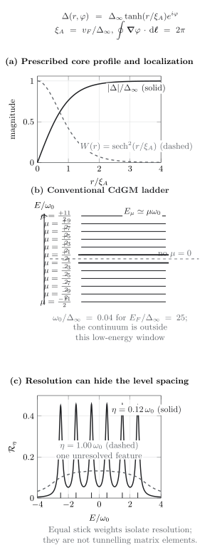
Controlled schematic for a clean, singly quantized conventional $s$-wave vortex in the quasiclassical regime. The prescribed tanh profile suppresses the pair field and localizes quasiparticle weight in the core. Its asymptotic levels occur in particle–hole-related pairs $E_\mu\simeq\mu\omega_0$, with half-integer $\mu$ and $\omega_0\sim\Delta_\infty^2/E_F$; there is no protected zero in this conventional ladder. The final panel convolves equal-weight spectral sticks only to demonstrate resolution: $\eta$ comparable to $\omega_0$ can make ordinary levels look like one central feature. It is not material data, a physical lifetime, or a calculated tunnelling LDOS.

Download the vortex diagnostic as SVG, inspect the radial profile, level ladder, and resolution curves, or read the semantic record.

The vortex page owns winding and long-distance energetics. The topological BdG page adds symmetry class, a bulk or defect invariant, and boundary or vortex matching before a protected zero mode can be claimed.

Validity ceilings beyond diagonalization

Finite size. The mesh must resolve the shortest wavelength used by the model, while the box must exceed every localization or coherence scale relevant to the conclusion. Separate a physical splitting from the eigensolver residual and the plotting broadening, and show a sequence in mesh and box size.

Disorder. Scalar disorder preserves intrinsic BdG particle–hole redundancy realization by realization, although it can break spatial or time-reversal symmetries. If $\Delta$ is self-consistent, solve it for each realization. Statistical claims report the ensemble, number of realizations, seeds, distribution or quantiles, and sample-to-sample uncertainty; a result about one specified realization should be labeled as sample-specific.

Charging and exact number. BdG is a broken-symmetry grand-canonical saddle. If the charging scale or exact number and parity constraints compete with the gap or level splitting, add the island term $E_C(\hat N-n_g)^2$ and perform the required number or parity projection. BdG eigenvalues alone are not the island’s many-body addition spectrum.

State identity. A local spectral peak establishes a feature of the declared quadratic saddle. Assigning it to a unique quasiparticle mechanism requires comparison with competing pair profiles, boundary models, disorder realizations, and open-system couplings. A zero-energy feature needs still stronger topological and experimental tests.

The shared chapter diagram places this method in the larger inference chain without replacing any of these local checks.

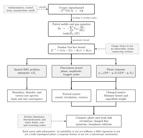
BdG theory maps an inhomogeneous saddle to spectra and local amplitudes after regulator, gauge, and boundary conditions are fixed. A subgap eigenvalue alone does not identify its origin. Original schematic, not to scale.

Read the chapter map’s semantic record. The paired-matter claim test matrix lists the additional controls needed for vortex, topological, and platform conclusions.

Diagnostics and stop conditions

Choose tolerances before looking at the desired low-energy feature. In the table, use the matrix spectral norm and the vector Euclidean norm, denoted by $\lVert\cdot\rVert_2$. Scale matrix norms by a declared energy $E_{\mathrm{ref}}$ and use the same regulator in every comparison.

Check	Required result	Stop condition
Hermiticity	$\lVert H-H^\dagger\rVert_2/E_{\mathrm{ref}}<\epsilon_H$ for a closed problem	Do not interpret eigenvalues or norms.
Particle–hole assembly	$\lVert\mathcal C H\mathcal C^{-1}+H\rVert_2/E_{\mathrm{ref}}<\epsilon_C$ on a $\mathcal C$-invariant domain	A basis, transpose, phase, or boundary condition is inconsistent.
Eigenpairs	$\lVert H\Psi_n-E_n\Psi_n\rVert_2/E_{\mathrm{ref}}<\epsilon_{\mathrm{eig}}$ and every state has its required partner	The claimed splitting is at or below unresolved solver error.
Norm and completeness	Orthonormality, global completeness, and each local LDOS sum rule pass	A truncated or duplicated state set is being used as complete.
Gauge covariance	A simultaneous transformation of hopping or $\mathbf A$, $\Delta$, $u$, and $v$ leaves energies and electron observables unchanged	The discretization or post-processing is gauge inconsistent.
Regulator and geometry	The feature converges in basis or mesh, box size, and matched cutoff	It moves on the same scale as the claimed physics.
Broadening	Conclusions survive a sequence of $\eta$ values and are separated from level spacing and temperature	A plotting resolution is being called a lifetime or gap.
Self-consistency	$R_\Delta$ and, if used, $R_N$ pass; the appropriate $\Omega$ or $F$ and the constrained Hessian are checked across distinct seeds	Iteration convergence or a lower functional value with a negative mode is insufficient.
Open-system spectrum	The retarded Green function has the required causality, positivity, particle–hole relation, and spectral-weight checks	A closed-box state is being reported as a device resonance.
Disorder inference	The stated sample-specific or statistical target matches the calculation and uncertainty summary	One favorable realization is being promoted to robustness or typicality.

Common pitfalls

Iteration convergence is not thermodynamic stability. A fixed-point solver can converge to a metastable or symmetry-restricted saddle. Compare multiple seeds with the same regulated free-energy functional.

Broadening is not a lifetime. Lorentzian plotting width can merge ordinary levels into one peak. A physical linewidth requires an open-system or interacting self-energy and a compatible measurement model.

A box state is not automatically a device resonance. Changing a wall into a lead changes the spectral problem from normalized eigenvectors to a retarded Green function with an energy-dependent self-energy.

A zero eigenvalue is not a Majorana identification. Particle–hole redundancy is present in every BdG problem. Protection needs the appropriate symmetry class, invariant, interface or defect, and finite-size tests.

One disorder realization is not an ensemble. It can establish a sample-specific counterexample or solution, but not a probability, typical value, or robustness claim.

Exercises

1. Recover the two-site spectrum and local sum rule

Starting from the displayed $4\times4$ matrix, eliminate three amplitudes in favor of $u_1$ and derive $\lambda^4-3\lambda^2+1=0$. Normalize the two positive-energy eigenvectors and recover the four LDOS weights at each site.

Solution

The eigenvalue equations are

$$-u_2=\lambda u_1, \quad -u_1+v_2=\lambda u_2, \quad v_2=\lambda v_1, \quad u_2+v_1=\lambda v_2.$$

Set $u_1=1$. Then $u_2=-\lambda$, $v_2=1-\lambda^2$, and $v_1=(1-\lambda^2)/\lambda$. The last equation gives $\lambda^4-3\lambda^2+1=0$, whose positive roots are $\varphi^{-1}$ and $\varphi$. Substitution gives the two displayed vectors. The unnormalized columns have squared norms $5-\sqrt5$ and $5+\sqrt5$, respectively, which gives the displayed normalization factors.

Reading the $u_i$ weights at positive energy and the $v_i$ weights at negative energy gives $a=(5+\sqrt5)/20$ and $b=(5-\sqrt5)/20$ in the displayed table. Since $a+b=1/2$, each local spectral integral is $2(a+b)=1$.

2. Check a lattice gauge transformation

For arbitrary site phases $\alpha_i$, show that $K'_{ij}=e^{i(\alpha_i-\alpha_j)}K_{ij}$ and $\Delta'_{ij}=e^{i(\alpha_i+\alpha_j)}\Delta_{ij}$ imply $H'=U_\alpha H U_\alpha^\dagger$. Explain why changing only the pair phase is not this gauge transformation.

Solution

Let $P_{ij}=e^{i\alpha_i}\delta_{ij}$ and $U_\alpha=\operatorname{diag}(P,P^\ast)$. Then

$$PKP^\dagger=K', \qquad P\Delta P^T=\Delta',$$

and direct block multiplication gives

$$U_\alpha \begin{pmatrix}K&\Delta\\\Delta^\dagger&-K^\ast\end{pmatrix} U_\alpha^\dagger =\begin{pmatrix}K'&\Delta'\\\Delta'^\dagger&-K'^\ast\end{pmatrix}.$$

Unitary equivalence preserves energies and norms, while the component phases preserve every $\lvert u_i\rvert^2$ and $\lvert v_i\rvert^2$. Changing $\Delta$ without the hopping phases changes the gauge-invariant phase gradient or boundary twist, so it describes different input data.

3. Separate a fixed point from a stable saddle

Suppose two initial pair fields converge below the same $R_\Delta$ tolerance but approach different final profiles. What must be compared before selecting one, and what extra equation is required if the total particle number is fixed?

Solution

Both profiles are legitimate fixed points of the numerical update, but iteration convergence does not order their thermodynamic stability. Evaluate the same regulated mean-field functional that generated the gap equation, with identical cutoff matching, normal-ordering terms, Hartree treatment, ensemble, and boundary conditions. At fixed $\mu$, compare $\Omega$ and test the Hessian on fixed-$\mu$ variations. The lowest branch among the locally stable solutions found is preferred within the declared mean-field approximation, but the search does not prove that no lower branch exists.

At fixed total number, also impose

$$N_{\mathrm{target}}=\int\mathrm d^d r\,n(\mathbf r)$$

and solve for $\mu$ together with $\Delta$ on each branch. Then compare $F=\Omega+\mu N$ and test the Hessian on variations that preserve $N$. Holding the normal-state $\mu$ fixed would silently change the ensemble.

Continue

Phase, amplitude, and Leggett modes studies two-particle fluctuation poles rather than BdG eigenvalues. Vortices and topological defects develops winding and long-distance defect energetics, while this page owns microscopic core spectra. Topological BdG superconductors adds symmetry class and bulk or defect invariants. Majorana evidence standards asks whether a real platform discriminates topological modes from ordinary Andreev, Kondo, disorder, and device alternatives.

References

• Andreev, A. F. (1964). “The thermal conductivity of the intermediate state in superconductors.” Soviet Physics JETP 19(5), 1228–1231. Open PDF.
• Caroli, C., de Gennes, P. G., and Matricon, J. (1964). “Bound fermion states on a vortex line in a type II superconductor.” Physics Letters 9, 307–309. doi:10.1016/0031-9163(64)90375-0.
• de Gennes, P. G. (1999). Superconductivity of Metals and Alloys. Westview Press, ch. 5. Publisher record.
• Gygi, F., and Schlüter, M. (1991). “Self-consistent electronic structure of a vortex line in a type-II superconductor.” Physical Review B 43, 7609–7621. doi:10.1103/PhysRevB.43.7609.
• Zhu, J.-X. (2016). Bogoliubov-de Gennes Method and Its Applications. Lecture Notes in Physics 924. Springer. doi:10.1007/978-3-319-31314-6.