Nonequilibrium, Driven, and Open Quantum Matter

Nonequilibrium quantum matter is defined by a protocol and an observation window, not by a Hamiltonian alone. A quench, ramp, periodic drive, kinetic constraint, bath, or measurement record can produce relaxation, scaling, temporal order, exceptional revivals, fragmented motion, or an open steady state. The central task is to identify which mechanism controls the signal and how long the resulting claim remains valid.

Helpful background. Quenches and relaxation introduces the model protocols used throughout, while equilibration, thermalization, and dephasing supplies the universal distinctions among stationary and thermal behavior.

Enter this chapter

Every analysis in this chapter declares six objects before assigning a dynamical label:

1. the initial density operator and how it was prepared;
2. the Hamiltonian, drive cycle, or open-system generator;
3. exact and approximate conserved quantities, including the selected symmetry or Krylov sector;
4. the observable and its detector or numerical reconstruction;
5. system size, boundary conditions, bath, and control errors; and
6. the interval over which the conclusion is asserted.

The chapter applies the general dynamical formalisms developed elsewhere to concrete quantum-matter models. It does not rederive Keldysh contours, the eigenstate thermalization hypothesis, Floquet prethermal theorems, or Lindblad field theory. Its job is to connect those structures to model observables and to stop each conclusion at the first untested timescale, size, or environmental assumption.

Useful maps of the neighboring formalisms are the reviews of closed-system nonequilibrium dynamics by Polkovnikov et al. 2011, high-frequency Floquet dynamics by Bukov, D’Alessio, and Polkovnikov 2015, Loschmidt transitions by Heyl 2018, scars and fragmentation by Moudgalya, Bernevig, and Regnault 2022, driven-open Keldysh theory by Sieberer, Buchhold, and Diehl 2016, and discrete time crystals by Zaletel et al. 2023. These sources organize distinct mechanisms; none licenses transferring a conclusion across protocols without the six declarations above.

The first map shows how four common experimental preparations lead to distinct mathematical objects and evidence claims. Follow a row from left to right; moving vertically changes the mechanism and therefore the decisive negative test.

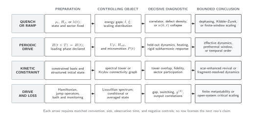
Protocol-to-claim dictionary for this chapter. Each row identifies the controlling mathematical object, representative observable, and strongest bounded conclusion; arrows denote inference, not automatic implication. The diagram is schematic and not to scale.

The route through the chapter is cumulative:

• Quenches and relaxation separate dephasing, equilibration, generalized ensembles, and thermalization in finite and infinite systems.
• Kibble–Zurek scaling derives freeze-out time, length, and defect laws for finite-rate critical ramps.
• Nonthermal fixed-point realizations test temporal scaling collapse and conservation-compatible transport in quantum gases.
• Floquet engineering keeps effective Hamiltonian, micromotion, resonances, loading, and heating in one controlled description.
• Floquet phases and time crystals add rigidity, correlations, lifetime, and size trends to a subharmonic response.
• Quantum-scar models connect exceptional eigenstates and special-state overlap to revivals in otherwise thermal spectra.
• Hilbert-space fragmentation constructs exact Krylov sectors and tests thermalization within them.
• Driven-dissipative cavity and circuit matter distinguishes finite-system metastability from a closing Liouvillian gap.
• Dynamical phase transitions derives Loschmidt critical times and limits their relation to local order.
• Heating, finite-size, and open-system evidence combines the clocks and negative controls into a final comparison.

One observation window, several ceilings

The same time trace can have several plausible explanations. The second figure makes the necessary time ordering explicit. Inspect the central interval first, then ask which upper bound is smallest in the system at hand.

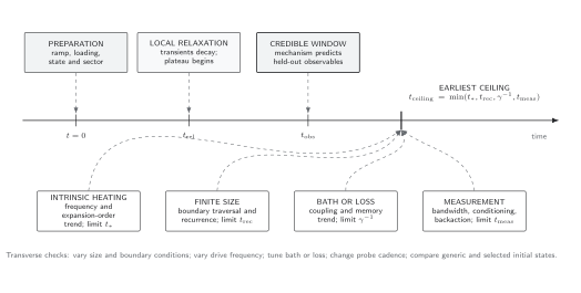
Validity and failure map for a finite driven or quenched system. The useful interval lies after preparation and local relaxation and before the earliest independently measured ceiling. Heating, recurrence, bath coupling, and measurement effects are competing explanations rather than interchangeable decay constants. Schematic and not to scale.

For a prethermal claim the desired hierarchy is $t_{\mathrm{rel}}\ll t_{\mathrm{obs}}\ll t_*$. For a finite device it must be strengthened to

$$t_{\mathrm{rel}}\ll t_{\mathrm{obs}} \ll \min\!\left(t_*,t_{\mathrm{rec}},\gamma^{-1},t_{\mathrm{meas}}\right).$$

Here $t_*$ is the intrinsic prethermal or heating scale, $t_{\mathrm{rec}}$ a relevant finite-size recurrence scale, $\gamma^{-1}$ an environmental lifetime, and $t_{\mathrm{meas}}$ the first time at which measurement resolution or backaction invalidates the unperturbed interpretation. Their numerical values must be obtained independently whenever possible.

Regime comparison

Together with the preceding prose and figure alternatives, the table gives a compact nonvisual account and a checklist for choosing a page. “Lifetime trend” means the trend predicted by the proposed mechanism; absence of that trend lowers the conclusion.

Regime	Protocol and controlling object	Primary observable	Expected lifetime or size trend	Main alternative	Strongest bounded claim
Dephasing	Sudden quench; post-quench energy gaps	Local correlator or imbalance	Stationary fluctuations shrink with effective dimension; recurrences move with size	Coarse time resolution	Observable equilibrates over a declared window
Kibble–Zurek production	Critical ramp; $\hat t$ and $\hat\xi$	Defect density or correlation length	Power law in ramp time, then finite-size saturation	Post-ramp coarsening	Freeze-out scaling in an independently fixed critical window
Nonthermal fixed point	Far-from-equilibrium quench; scaling function	$n(k,t)$ collapse and transported invariant	Scaling range widens before infrared or ultraviolet cutoff	Transient redistribution or imaging convolution	Finite-window self-similar dynamics
Floquet engineering	Periodic drive; $H_{\mathrm{eff}}$ plus micromotion	Held-out stroboscopic and intraperiod observables	Error decreases with expansion order until resonances or noise dominate	Calibrated single-particle dressing only	Engineered dynamics within a prethermal window
Discrete time crystal	Periodic drive; quasienergy pairing or prethermal symmetry breaking	Rigid subharmonic correlations	Lifetime grows with size or drive frequency according to mechanism	Beat note, synchronization, or recurrence	Robust finite-window temporal order
Many-body scars	Special quench; exceptional spectral tower	State-selective fidelity and local revival	Tower reconstruction and perturbation trend persist with size	Accidental commensurability	Scar-enhanced revival dynamics in a specified model
Hilbert-space fragmentation	Kinetic constraint; Krylov connectivity graph	Sector participation and memory	Exact sectors remain disconnected; weak breaking gives coupling-dependent leakage	Disorder localization or slow energetics	Fragment-resolved dynamics or a prefragmented window
Driven-dissipative criticality	Coherent drive and loss; Liouvillian	Output correlations and relaxation gap	Gap closes only in a declared large-system or large-occupation limit	Finite-system switching	Metastability or open critical scaling, as tested
Loschmidt transition	Global quench; return-rate Fisher zeros	Return probability and critical-time scaling	Rounding sharpens with size	Smooth local crossover	Dynamical return-rate criticality
Bath- or measurement-limited behavior	Drive or quench plus environment; channel or memory kernel	Unconditional and conditional records	Rate follows bath coupling, probe cadence, or memory time	Intrinsic heating	Environment-bounded nonequilibrium response

Cross-chapter distinctions

Several neighboring concepts share signatures but not definitions. A scar is a special spectral subset inside a broadly connected symmetry block; fragmentation is a decomposition of that block into invariant Krylov sectors. A time crystal is rigid collective temporal order; a scar revival can be long lived and periodic without breaking discrete time translation. A Loschmidt singularity concerns a global overlap; a dissipative phase transition concerns the steady-state spectrum of a generator. Nonthermal fixed-point scaling concerns attraction of distributions under evolution; a stationary turbulent cascade concerns flux maintained through scales.

These distinctions are operational. They tell the reader which perturbation, size scan, initial-state comparison, or ensemble construction can falsify the proposed label.

Chapter project

Choose one finite driven spin chain or bosonic lattice. Compute exact one-period evolution for at least three sizes, compare it with a truncated effective Hamiltonian, and prepare both a structured and a generic initial state. Record energy absorption, a local correlator, return probability, and participation in any proposed Krylov or scar subspace. Add either a weak constraint-breaking term or a calibrated Lindblad channel. The final result must state which observed plateau or revival survives frequency, size, initial-state, and environment tests.

A reproducible verification workflow is the executable home for that comparison. Mutable claims, new platform results, and contrary evidence are maintained in the Quantum Matter and Emergence Research dossier. Neither interface changes the mathematical definitions given in the chapter.

Review the chapter

1. Classify a revival. A 20-site driven chain shows a sharp period-doubled peak for 80 cycles from one Néel state. List the minimum additional tests needed before calling it a discrete time crystal rather than a scar-assisted or finite-size revival.

Solution

Vary pulse error over a finite interval to test frequency locking; measure unequal-time correlations; compare several sizes and generic or symmetry-related initial states; extract lifetime using a fixed threshold; independently measure heating, decoherence, and traversal scales; and perturb the proposed stabilization mechanism. A scar explanation is favored if only a narrow initial-state family overlaps an exceptional tower. A recurrence is favored if revival time follows boundary traversal or small-spectrum commensurability without a rigidity interval.

2. Order the limits. Explain why a finite isolated system can have an exact long-time average while lacking a literal stationary state at every late time.

Solution

Finite unitary dynamics is a quasiperiodic sum of discrete frequencies. Its time average can exist because oscillatory off-diagonal terms average away, yet the instantaneous state continues to evolve and eventually recurs arbitrarily closely. A relaxation statement for local observables generally takes the thermodynamic limit before the late-time limit or asserts only a finite observation window.

References

• Bukov, Marin, Luca D’Alessio, and Anatoli Polkovnikov. “Universal High-Frequency Behavior of Periodically Driven Systems: From Dynamical Stabilization to Floquet Engineering.” Advances in Physics 64, 139–226 (2015). DOI.
• Heyl, Markus. “Dynamical Quantum Phase Transitions: A Review.” Reports on Progress in Physics 81, 054001 (2018). DOI.
• Moudgalya, Sanjay, B. Andrei Bernevig, and Nicolas Regnault. “Quantum Many-Body Scars and Hilbert Space Fragmentation: A Review of Exact Results.” Reports on Progress in Physics 85, 086501 (2022). DOI.
• Polkovnikov, Anatoli, Krishnendu Sengupta, Alessandro Silva, and Mukund Vengalattore. “Colloquium: Nonequilibrium Dynamics of Closed Interacting Quantum Systems.” Reviews of Modern Physics 83, 863–883 (2011). DOI.
• Sieberer, Lukas M., Michael Buchhold, and Sebastian Diehl. “Keldysh Field Theory for Driven Open Quantum Systems.” Reports on Progress in Physics 79, 096001 (2016). DOI.
• Zaletel, Michael P., Mikhail Lukin, Christopher Monroe, Chetan Nayak, Frank Wilczek, and Norman Y. Yao. “Colloquium: Quantum and Classical Discrete Time Crystals.” Reviews of Modern Physics 95, 031001 (2023). DOI.