Fermi-Liquid Response and Zero Sound

In a neutral or screened three-dimensional Fermi liquid, the same forward-scattering parameters that set the equilibrium compressibility and spin susceptibility also reshape the dynamical particle–hole response. A sufficiently repulsive density interaction pulls a collective pole above the particle–hole continuum: zero sound. The result is simple only after the route toward $(q,\omega)=(0,0)$, the response convention, and the collision hierarchy have all been specified.

Required background. Use Landau theory for the quasiparticle interaction and total-density-of-states convention, and the Kubo-response framework for retarded correlators. Helpful background. The Ward-consistent response and diffusion, conductivity, and susceptibility pages explain why conservation laws distinguish the limits below.

Four paths to the origin give four observables

Assume an isotropic, spin-rotation-invariant normal Fermi liquid at low temperature. Let $N(0)$ be the total two-spin quasiparticle density of states at the Fermi surface, $v_F^*$ the quasiparticle Fermi velocity, and $\tau_{\mathrm{coll}}$ the relaxation time of the nonconserved angular distortions relevant to the longitudinal mode. The small-$q$, small-$\omega$ plane contains several physically different experiments:

Probe	Limiting path or hierarchy	Leading density result
Equilibrium compression	$\omega\to0$ before $q\to0$	$\mathcal R_s=N(0)/(1+F_0^s)$
Spatially uniform drive	$q\to0$ at nonzero $\omega$	$\mathcal R_s=0$ by number conservation
Collisionless ray	$q,\omega\to0$ at fixed $z=(\omega+i0^+)/(qv_F^*)$ and $\omega\tau_{\mathrm{coll}}\gg1$	Particle–hole continuum and possible zero-sound pole
Hydrodynamic ray	$q,\omega\to0$ with $\omega\tau_{\mathrm{coll}}\ll1$	First sound in a clean neutral fluid

Thus zero sound is neither of the two iterated limits. At any fixed nonzero temperature, taking $q\to0$ along $\omega\propto q$ eventually makes $\omega\tau_{\mathrm{coll}}\ll1$; the strict infrared mode is then hydrodynamic. The collisionless limit instead keeps

$$q\ll k_F, \qquad \tau_{\mathrm{coll}}^{-1}\ll\omega=sqv_F^*\ll E_F, \qquad q\ell_{\mathrm{coll}}\gg1,$$

with $\ell_{\mathrm{coll}}=v_F^*\tau_{\mathrm{coll}}$. One may reach this window by lowering the temperature before taking the long-wavelength limit.

The two panels below separate collisionless spectral kinematics from the paths used to approach the origin. In panel (a), inspect the narrow gap between the one-pair edge and the $F_0^s=1$ zero-sound ray. In panel (b), notice that at fixed finite $\tau_{\mathrm{coll}}$ the collisionless route stops before the crossover, whereas the hydrodynamic route reaches the origin.

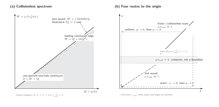
Small-$q$ response of a neutral or statically screened, isotropic three-dimensional Fermi liquid. The hatched region in panel (a) is the leading collisionless one-particle–one-hole continuum, $0<\omega<qv_F^*$; the displayed $F_0^s=1$ zero-sound root is $s_0=1.044382$ and lies just above its edge. More generally, the $F_0^s$-only kernel has a separated real root $s_0>1$ for $F_0^s>0$ in the collisionless hierarchy $\omega\tau_{\mathrm{coll}}\gg1$. Panel (b) shows why static, uniform, collisionless, and hydrodynamic approaches to $(q,\omega)=(0,0)$ are inequivalent. First sound belongs to $\omega\tau_{\mathrm{coll}}\ll1$ and is not a pole of the collisionless kernel; its possible location inside the collisionless one-pair wedge does not by itself imply collisionless Landau damping. The figure is schematic apart from the equation-checked slope ratio in panel (a), and it omits recoil, thermal and multipair broadening, lattice anisotropy, and the unscreened Coulomb plasmon.

Hatching denotes continuum support, the heavy solid ray denotes zero sound, dash–dot denotes first sound, and the pale dotted band denotes a collision crossover rather than a phase boundary. The downloadable SVG and machine-readable semantic record preserve the visual and scientific distinctions.

For orientation, the chapter’s validity and failure map places this response calculation among its microscopic inputs and instabilities, while the claim table states the assumptions behind the principal Fermi-liquid formulas.

Sources and static response fix the signs

Define density and spin-number channels by

$$n_s=n_\uparrow+n_\downarrow, \qquad n_a=n_\uparrow-n_\downarrow,$$

and couple sources through

$$H_U=H_0-\int d^3x\,[U_s n_s+U_a n_a].$$

With the site’s convention

$$G_c^R(t,\mathbf x) =-i\theta(t)\langle[n_c(t,\mathbf x),n_c(0)]\rangle, \qquad c=s,a,$$

the physical response is $\mathcal R_c=\delta n_c/\delta U_c=-G_c^R$. This minus sign is worth making explicit: the static physical response is positive. In the total-DOS convention,

$$\lim_{q\to0}\lim_{\omega\to0}\mathcal R_s(q,\omega) =\frac{N(0)}{1+F_0^s} =n^2\kappa_T,$$ $$\lim_{q\to0}\lim_{\omega\to0}\mathcal R_a(q,\omega) =\frac{N(0)}{1+F_0^a}.$$

If $U_a=\mu_{\mathrm{mag}}B$ and $M=\mu_{\mathrm{mag}}n_a$, then $\chi_M=\mu_{\mathrm{mag}}^2\mathcal R_a$. A convention using $S_z=n_a/2$ instead has the corresponding factor of $1/4$. The divergences at $F_0^s=-1$ and $F_0^a=-1$ mark density and ferromagnetic Pomeranchuk instabilities, respectively. These thermodynamic relations follow from varying the Landau energy functional; see Dupuis 2025, § 4.2.2–4.2.3, pp. 296–297.

The kinetic equation transports a surface deformation

Choose $\mathbf q$ as the polar axis, write $\mu=\hat{\mathbf p}\cdot\hat{\mathbf q}$, and parametrize a Fermi-surface displacement by

$$\delta n_{\mathbf p\sigma} =-\frac{\partial n_0}{\partial\epsilon_{\mathbf p}} \bigl[\nu^s(\mu)+\sigma\nu^a(\mu)\bigr] e^{i(\mathbf q\cdot\mathbf r-\omega t)}, \qquad \sigma=\pm1.$$

The dimensionless Landau functions are

$$F^c(\hat{\mathbf p}\cdot\hat{\mathbf p}') =N(0)f^c(\hat{\mathbf p}\cdot\hat{\mathbf p}') =\sum_{\ell=0}^{\infty}F_\ell^c P_\ell(\hat{\mathbf p}\cdot\hat{\mathbf p}'), \qquad c=s,a.$$

Keeping only $F_0^c$ is a solvable truncation, not a claim that higher harmonics vanish in a real liquid. In this model the quasiparticle-energy shift is

$$\delta\epsilon_{\mathbf p\sigma} =F_0^s\bar\nu^s+\sigma F_0^a\bar\nu^a -U_s-\sigma U_a, \qquad \bar\nu^c=\frac12\int_{-1}^{1}\nu^c(\mu)\,d\mu.$$

The linearized Landau–Boltzmann equation is

$$\left( \partial_t+\mathbf v_{\mathbf p}^*\cdot\nabla_{\mathbf r} \right)\delta n_{\mathbf p\sigma} -\frac{\partial n_0}{\partial\epsilon_{\mathbf p}}\, \mathbf v_{\mathbf p}^*\cdot\nabla_{\mathbf r} \delta\epsilon_{\mathbf p\sigma} =I_{\mathrm{coll}}[\delta n].$$

Dropping its collision integral in the hierarchy above reduces it to one equation per channel,

$$(z-\mu)\nu^c(\mu) =\mu\bigl[F_0^c\bar\nu^c-U_c\bigr], \qquad z=\frac{\omega+i0^+}{qv_F^*}.$$

This equation says something geometrically simple: quasiparticles with velocity component $\mu v_F^*$ stream the angular distortion, while the mean field $F_0^c\bar\nu^c$ tries to make the whole Fermi surface move coherently. Landau’s original derivation proceeds from the full kinetic equation to this angular eigenproblem in Landau 1957, printed pp. 102–103, Eqs. (4)–(14).

The angular integral exposes the continuum and the pole

Solving for $\nu^c(\mu)$ and averaging once gives

$$\bar\nu^c =\Phi(z)\bigl[F_0^c\bar\nu^c-U_c\bigr],$$

where

$$\Phi(z) =\frac12\int_{-1}^{1}\frac{\mu\,d\mu}{z-\mu} =\frac{z}{2}\log\left(\frac{z+1}{z-1}\right)-1.$$

The retarded logarithm is analytic for $\operatorname{Im}z>0$ and is real for $z>1$. Since $\delta n_c=N(0)\bar\nu^c$, the correlator and physical response are

$$G_c^R(q,\omega) =N(0)\frac{\Phi(z)}{1-F_0^c\Phi(z)}, \qquad \mathcal R_c(q,\omega) =-N(0)\frac{\Phi(z)}{1-F_0^c\Phi(z)}.$$

Two immediate checks recover the first table: $\Phi(0)=-1$ gives the static susceptibility, whereas $\Phi(z\to\infty)\to0$ makes the uniform finite-frequency density response vanish.

For $0<s<1$, the upper rim of the retarded branch cut is

$$\Phi(s+i0^+) =\frac{s}{2}\log\left(\frac{1+s}{1-s}\right) -1-\frac{i\pi s}{2}.$$

This cut is the linearized particle–hole continuum, $0<\omega<qv_F^*$ at positive frequency. The leading edge $qv_F^*$ is universal at small $q$, but its $O(q^2)$ correction depends on the curvature of the quasiparticle dispersion; for a strictly quadratic dispersion it is $q^2/(2m^*)$. The Lindhard-response page displays this recoil explicitly. At $T=0$ and positive frequency, use the same spectral normalization as that page:

$$S_c(q,\omega) =-2\operatorname{Im}G_c^R(q,\omega) =2\operatorname{Im}\mathcal R_c(q,\omega).$$

The continuum weight is manifestly positive:

$$S_c^{\mathrm{cont}}(q,\omega) =\frac{N(0)\pi s} { [1-F_0^c\operatorname{Re}\Phi(s)]^2 +[\pi F_0^c s/2]^2 }, \qquad 0<s<1.$$

At fixed $q$, a density probe therefore sees a broad particle–hole continuum plus, when it is separated, the sharp collective peak derived next. At finite temperature, $-2\operatorname{Im}G_c^R$ remains the spectral density, but the unsymmetrized structure factor contains detailed balance:

$$\mathcal S_c^>(q,\omega) =\frac{-2\operatorname{Im}G_c^R(q,\omega)} {1-e^{-\beta\omega}}.$$

The response function, continuum, and collective contribution are derived together in Dupuis 2025, § 4.3.4.1, printed pp. 305–307, Eqs. (4.100)–(4.108).

The zero-sound pole has a computable residue

A source-free density oscillation requires the denominator to vanish:

$$1=F_0^s\Phi(s_0), \qquad s_0>1, \qquad \omega_0(q)=s_0qv_F^*.$$

For every $F_0^s>0$, $\Phi(s)$ decreases monotonically from $+\infty$ at $s=1^+$ to $0$ at infinity, so there is one real root above the one-pair continuum. It is undamped only within the collisionless, linearized, single-pair theory. Collisions, thermally excited quasiparticles, multipair states, and finite-$q$ curvature can all broaden or obscure it.

The pole’s weight is not determined by its speed. Since

$$\Phi'(s) =\frac12\log\left(\frac{s+1}{s-1}\right) -\frac{s}{s^2-1}<0 \qquad (s>1),$$

the pole part of the correlator is

$$G_{s,\mathrm{pole}}^R(q,\omega) =\mathcal Z_0(q) \left[ \frac1{\omega-\omega_0+i0^+} -\frac1{\omega+\omega_0+i0^+} \right],$$

with positive collective-response residue

$$\mathcal Z_0(q) =-\frac{N(0)qv_F^*} {(F_0^s)^2\Phi'(s_0)}>0.$$

This derivative formula is the long-wavelength form of Dupuis 2025, printed pp. 306–307, Eq. (4.108).

This $\mathcal Z_0$ is not the one-particle quasiparticle residue conventionally called $Z$. At $T=0$ and positive frequency the pole contributes

$$S_s^{\mathrm{pole}}(q,\omega) =2\pi\mathcal Z_0(q)\delta(\omega-\omega_0).$$

For example, $F_0^s=1$ gives

$$s_0=1.044382\ldots, \qquad \frac{\mathcal Z_0(q)}{N(0)qv_F^*} =0.104217\ldots.$$

The limiting forms provide strong diagnostic checks:

$$s_0-1 =2\exp\left[-2\left(1+\frac1{F_0^s}\right)\right] [1+o(1)], \qquad 0<F_0^s\ll1,$$ $$s_0^2 =\frac{F_0^s}{3}+\frac35 +O\bigl((F_0^s)^{-1}\bigr), \qquad F_0^s\gg1.$$

At weak coupling the pole exists but is exponentially close to the continuum and has exponentially small weight. Resolving it requires the separation $(s_0-1)qv_F^*$ to exceed collision broadening, thermal smearing, and the recoil correction. Landau 1957, printed pp. 103–104 and Dupuis 2025, p. 302, Eqs. (4.83)–(4.84) give the pole equation and leading weak- and strong-coupling limits; the subleading $3/5$ above follows by expanding the same equation one order further.

For a stable attractive channel, $-1<F_0^s\le0$, there is no separated real pole above the continuum in this truncation. Any pole obtained by continuing through the branch cut lies on an unphysical sheet and is damped; it must not be described as a real undamped mode “inside” the continuum. At $F_0^s<-1$, an upper-half-plane mode instead diagnoses instability of the assumed normal state. See Dupuis 2025, § 4.3.3.1, printed p. 302.

Spin modes and higher harmonics change the eigenproblem

In an exactly spin-rotation-invariant liquid, the same derivation applies to the spin-number response after $F_0^s\to F_0^a$. An undamped $F_0$-only spin-zero-sound pole therefore requires $F_0^a>0$. The common range $-1<F_0^a<0$ enhances the static spin response but leaves the collective feature in the particle–hole continuum; $F_0^a\to-1^+$ approaches a ferromagnetic instability. Spin–orbit, dipolar, and other spin-relaxation processes add decay, and the hydrodynamic spin mode is generally diffusive rather than ordinary first sound. Landau gives the corresponding spin kinetic equation in Landau 1957, printed p. 107, Eqs. (25)–(29).

When $F_{\ell>0}^c$ is retained, $\nu^c(\hat{\mathbf p})$ must be expanded in angular harmonics and the kinetic equation becomes a matrix eigenvalue problem. Higher harmonics can shift the mode speed, redistribute spectral weight, and create additional angular collective modes. The one-line $F_0$ pole equation is then no longer the complete dispersion relation.

Conservation requires the matching current vertex

At large $z$, the $F_0$ response has

$$\Phi(z)=\frac1{3z^2}+\frac1{5z^4}+O(z^{-6}),$$

so

$$G_s^R(q,\omega) =\frac{N(0)(v_F^*)^2q^2}{3\omega^2} +O\left(\frac{q^4}{\omega^4}\right).$$

The explicit $q^2$ verifies that a spatially uniform scalar drive cannot change a conserved total particle number. For a spherical Fermi surface, however, the displayed coefficient is $n/m^*$. A Galilean-invariant system must instead have $n/m$ and obey

$$\int_0^\infty \frac{d\omega}{2\pi}\, \omega S_s(q,\omega) =\frac{nq^2}{2m}.$$

The missing factor is supplied by the $F_1^s$ current vertex and quasiparticle backflow. The Galilean Ward identity

$$1+\frac{F_1^s}{3}=\frac{m^*}{m}$$

restores the bare-mass coefficient. Thus the $F_0$ model is a controlled illustration of the density pole, but it is not a complete Galilean-invariant current response when $m^*\ne m$. On a lattice, the corresponding optical or stress sum rule replaces $n/m$, and interband or incoherent weight may be essential. The Ward-response page develops this vertex logic in general.

Collisions turn zero sound into first sound

The collisionless equation discarded $I_{\mathrm{coll}}[\delta n]$ from the Landau–Boltzmann equation. In a clean neutral fluid, a usable collision operator must conserve particle number, momentum, and energy:

$$\sum_{\mathbf p\sigma}I_{\mathrm{coll}}=0, \qquad \sum_{\mathbf p\sigma}\mathbf p\,I_{\mathrm{coll}}=0, \qquad \sum_{\mathbf p\sigma}\epsilon_{\mathbf p}I_{\mathrm{coll}}=0.$$

A naive replacement $\omega\to\omega+i/\tau_{\mathrm{coll}}$ does not enforce these constraints and cannot be trusted to produce the hydrodynamic limit. A relaxation-time model must project out the local-equilibrium density, momentum, and energy modes. This issue is explicit in Abrikosov and Khalatnikov 1958, § 9, printed p. 79.

When $\omega\tau_{\mathrm{coll}}\ll1$, collisions establish local equilibrium and the longitudinal density mode becomes first sound. Its speed is $c_1^2=(mn\kappa_S)^{-1}$, where $\kappa_S$ is the adiabatic compressibility. Using the $T\to0$ thermodynamic coefficients of a clean, neutral, Galilean-invariant liquid—while retaining a small nonzero temperature or another momentum-conserving equilibration mechanism so that the hydrodynamic hierarchy still holds—gives

$$c_1^2 =\frac{(v_F^*)^2}{3} (1+F_0^s)\left(1+\frac{F_1^s}{3}\right),$$

and, before dissipative corrections,

$$\mathcal R_s^{\mathrm{hyd}}(q,\omega) =\frac{nq^2/m} {c_1^2q^2-(\omega+i0^+)^2}.$$

At strictly $T=0$ in a clean normal Fermi liquid, $\tau_{\mathrm{coll}}^{-1}\to0$ and this hydrodynamic window closes; $c_1$ is the $T\to0$ hydrodynamic extrapolation.

First and zero sound solve different eigenproblems, so their speeds need not agree. For example, $F_0^s=1$ and $F_1^s=0$ give

$$\frac{c_1}{v_F^*}=\sqrt{\frac23}=0.816497\ldots, \qquad \frac{c_0}{v_F^*}=s_0=1.044382\ldots.$$

There is no contradiction in the first-sound speed lying inside the collisionless one-pair wedge: frequent collisions have already reorganized the dynamics into local equilibrium, and hydrodynamic attenuation is controlled by transport coefficients rather than collisionless Landau damping.

Viscosity and thermal conduction add sound attenuation. The intermediate regime $\omega\tau_{\mathrm{coll}}\sim1$ is often strongly damped and requires the full collision integral. The relevant angular-harmonic relaxation rates scale as $T^2/E_F$ at low temperature, with probe-frequency corrections of order $\omega^2/E_F$ and channel-dependent coefficients; they need not equal the on-shell one-particle lifetime. Cooling at fixed probe frequency can therefore drive first sound into zero sound, although pairing may intervene first. Landau 1957, printed p. 105 separates the hydrodynamic, crossover, and collisionless regimes, while Dupuis 2025, § 4.3.3.2, printed pp. 303–304 gives the first-sound speed in the present convention.

Where the acoustic pole survives

The derivation above assumes short-range or statically screened interactions, a smooth three-dimensional Fermi surface, a normal state, and a probe inside the Landau window. Several changes alter the conclusion:

• In a three-dimensional charged fluid with unscreened Coulomb interactions, the longitudinal density oscillation is lifted to a gapped plasmon; see Silin 1959, printed p. 872, Eqs. (18)–(20) and the plasmon page. In two dimensions with three-dimensional Coulomb fields, the long-wavelength plasmon instead scales as $\sqrt q$.
• On a lattice, momentum relaxation, Umklapp, and anisotropy can make the hydrodynamic density mode diffusive and turn the angular equation into a Fermi-surface integral rather than a Legendre problem.
• At finite temperature or disorder, a collisionless pole must be separated from both the continuum and its finite width. “Above the continuum” is not by itself an experimental visibility criterion.
• Near pairing, density-wave, or Pomeranchuk instabilities, the normal-state Landau parameters and collision kernel acquire strong scale dependence; the assumed normal Fermi liquid may fail before the formal pole is reached.

Common pitfalls

Taking limits without naming the path. Compressibility, a uniform dynamic response, zero sound, and first sound approach the same origin in the $(q,\omega)$ plane but are not interchangeable. State the order of limits and the size of $\omega\tau_{\mathrm{coll}}$ before interpreting a formula.

Calling every denominator zero an undamped mode. A real pole on the physical sheet above the one-pair continuum is different from a resonance reached through a branch cut. Also compare its separation and residue with all sources of broadening.

Using $v_F$ when the theory needs $v_F^*$. The kinetic equation transports quasiparticles, so its velocity is the interacting Fermi velocity. The bare mass reappears in a Galilean sum rule only after the matching current vertex and backflow are included.

Adding $i/\tau_{\mathrm{coll}}$ without conserving slow densities. This shortcut can erase the hydrodynamic zero modes of the collision operator. Projecting out the conserved local-equilibrium distortions is part of the approximation, not an optional refinement.

Exercises

1. Starting from $(z-\mu)\nu=\mu(F_0\bar\nu-U)$, derive the response $\mathcal R=-N(0)\Phi/(1-F_0\Phi)$. Check both iterated limits at the origin.

Solution

Solve for the angular distortion and average:

$$\bar\nu =(F_0\bar\nu-U) \frac12\int_{-1}^{1}\frac{\mu\,d\mu}{z-\mu} =\Phi(z)(F_0\bar\nu-U).$$

Therefore $\bar\nu/U=-\Phi/(1-F_0\Phi)$ and $\mathcal R=N(0)\bar\nu/U$. For $\omega\to0$ first, $z\to0$ and $\Phi\to-1$, giving $\mathcal R=N(0)/(1+F_0)$. For $q\to0$ at fixed nonzero $\omega$, $z\to\infty$ and $\Phi\to0$, giving $\mathcal R=0$.

2. Derive the weak- and strong-coupling limits of the zero-sound speed through the first nontrivial term.

Solution

For $s=1+\delta$ with $\delta\ll1$,

$$\Phi(1+\delta) =\frac12\log\frac{2}{\delta}-1+o(1).$$

Setting $F_0\Phi=1$ gives $\delta=2e^{-2(1+1/F_0)}[1+o(1)]$. For $s\gg1$, use

$$\Phi(s)=\frac1{3s^2}+\frac1{5s^4}+O(s^{-6}).$$

Writing $s^2=F_0/3+c+O(F_0^{-1})$ in $F_0\Phi=1$ yields $c=3/5$.

3. For $F_0^s=1$, verify the quoted speed and residue numerically, and explain why the residue is positive.

Solution

Solving $\Phi(s_0)=1$ for $s_0>1$ gives $s_0=1.044382\ldots$. At this point $\Phi'(s_0)<0$, so

$$\frac{\mathcal Z_0}{N(0)qv_F^*} =-\frac1{\Phi'(s_0)} =0.104217\ldots>0.$$

The sign is also required by the positive-frequency spectral weight

$$S_s^{\mathrm{pole}} =2\pi\mathcal Z_0\delta(\omega-\omega_0).$$

4. Show why an $F_0$-only model with $m^*\ne m$ misses the Galilean density $f$-sum coefficient, and identify the missing ingredient.

Solution

At large $z$, the model gives

$$G_s^R\simeq \frac{N(0)(v_F^*)^2q^2}{3\omega^2} =\frac{nq^2}{m^*\omega^2}.$$

The Galilean commutator sum rule requires $nq^2/(m\omega^2)$. The $\ell=1$ interaction dresses the current through quasiparticle backflow; using $1+F_1^s/3=m^*/m$ restores the required bare-mass coefficient and hence the $f$-sum rule.

5. Take $F_0^s=1$, $F_1^s=0$, and $qv_F^*=10^{-2}E_F$. Classify the response when (a) $\tau_{\mathrm{coll}}E_F=10$ and (b) $\tau_{\mathrm{coll}}E_F=10^3$. In case (b), use $\tau_{\mathrm{coll}}^{-1}$ as a broadening estimate and decide whether the zero-sound peak is cleanly separated from the continuum.

Solution

In case (a), the first-sound estimate gives

$$\omega\tau_{\mathrm{coll}} \simeq \sqrt{\frac23}\,(10^{-2})(10) =0.0816\ll1.$$

The probe is hydrodynamic, so first sound is the appropriate mode. In case (b), the collisionless zero-sound root gives

$$\omega_0\tau_{\mathrm{coll}} =s_0(10^{-2})(10^3) =10.44\gg1,$$

so the kinetic regime is collisionless. Nevertheless, its separation from the leading continuum edge is only

$$\Delta\omega =(s_0-1)qv_F^* =4.44\times10^{-4}E_F,$$

whereas the assumed broadening scale is $\tau_{\mathrm{coll}}^{-1}=10^{-3}E_F$. The response can satisfy $\omega_0\tau_{\mathrm{coll}}\gg1$ without showing a cleanly resolved peak; regime classification and experimental visibility are separate tests.

Continue

• Return to Landau theory for thermodynamics and stability.
• Compare the free particle–hole continuum on the Lindhard-response page.
• Connect the phenomenological parameters to the microscopic quasiparticle self-energy.
• Continue to plasmons and collective charge modes or to ideal hydrodynamic modes.

References

• A. A. Abrikosov and I. M. Khalatnikov, “Theory of the Fermi Fluid (The Properties of Liquid He³ at Low Temperatures),” Soviet Physics Uspekhi 1, 68–90 (1958), doi:10.1070/PU1958v001n01ABEH003086, Open PDF.
• Nicolas Dupuis, Field Theory of Condensed Matter and Ultracold Gases, Vol. 1 (World Scientific, 2023), ch. 4; updated chapter PDF, January 16, 2025, doi:10.1142/q0409, author PDF.
• L. D. Landau, “Oscillations in a Fermi Liquid,” Soviet Physics JETP 5, 101–108 (1957), official article, official PDF.
• V. P. Silin, “The Oscillations of a Degenerate Electron Fluid,” Soviet Physics JETP 8, 870–875 (1959), official PDF.

Further reading

• Gordon Baym and Christopher Pethick, Landau Fermi-Liquid Theory: Concepts and Applications, Wiley, New York (1991), ch. 1, doi:10.1002/9783527617159.