Scaling Dimensions, Correlators, and Critical Exponents

The previous page ended with the simplest continuum correlators of the critical Ising theory: free chiral Majorana fermions and the energy bilinear. This page steps back and explains the general logic behind those formulas. At a continuous phase transition, the correlation length is infinite, so the long-distance theory has no preferred scale. Local observables reorganize into scaling fields, and their correlation functions become homogeneous functions of the separations.

The central number attached to a scaling field is its scaling dimension. For the two-dimensional Ising spin field,

$$\langle \sigma(z_1,\bar z_1)\sigma(z_2,\bar z_2)\rangle ={C_\sigma\over |z_1-z_2|^{1/4}},$$

so the spin field has

$$\Delta_\sigma={1\over8}.$$

The spin dimension fixes the anomalous exponent and the critical isotherm. Together with the thermal correlation-length exponent, it also determines the magnetization and susceptibility exponents. The energy dimension fixes that correlation-length exponent and controls the singular specific heat. This page makes the operator-to-exponent dictionary precise, including its scaling assumptions and logarithmic exceptions.

Required background. Lesson 11 supplies the critical Ising spin, energy, and Majorana correlators used as the main examples.

Helpful background. Lesson 4 introduces critical power laws, and Lesson 5 develops RG eigenvalues and anomalous dimensions perturbatively.

Scaling fields

Scaling action and exponent notation

We work in Euclidean $d$ dimensions unless stated otherwise. In two dimensions,

$$z=x+iy, \qquad \bar z=x-iy, \qquad |z|^2=z\bar z.$$

A scalar scaling field $O(x)$ of dimension $\Delta_O$ is written in the convention

$$\mathcal D_\lambda O(x)\mathcal D_\lambda^{-1} =\lambda^{\Delta_O}O(\lambda x).$$

At a scale-invariant vacuum, this is equivalent to the correlator homogeneity law

$$\left\langle \prod_{i=1}^n O_i(\lambda x_i)\right\rangle = \lambda^{-\sum_i \Delta_i} \left\langle \prod_{i=1}^n O_i(x_i)\right\rangle.$$

The critical exponent for the correlation length is also traditionally called $\nu$. To avoid confusion, this page uses $\Delta$ for operator dimensions and $\nu$ only for the correlation-length exponent.

A microscopic lattice observable is usually not a pure scaling field. Instead, near a critical point it expands into a sum of continuum scaling fields:

$$O_{\rm lat}(i) \sim \sum_k c_k a^{\Delta_k} O_k(x), \qquad x=ai,$$

where $a$ is the lattice spacing. At long distance the term with the smallest scaling dimension compatible with the symmetries dominates.

For the Ising spin variable,

$$\sigma_i \sim c_\sigma a^{\Delta_\sigma}\sigma(x)+\cdots.$$

For the nearest-neighbor energy density, one first subtracts the expectation value in order to remove the identity operator:

$$E_i-\langle E\rangle \sim c_\epsilon a^{\Delta_\epsilon} \bigl(\epsilon(x)-\langle\epsilon\rangle\bigr)+\cdots.$$

The identity has dimension zero and contributes to one-point functions, but it is not the thermal perturbation that changes the critical theory. The energy field $\epsilon$ is the leading nontrivial scalar even under the Ising spin flip.

At the critical point, dilation acts diagonally on scaling fields:

$$O_i(x)\mapsto \lambda^{\Delta_i}O_i(\lambda x).$$

Away from the critical point the statement holds only inside the scaling window

$$a\ll |x|\ll \xi,$$

where $\xi$ is the correlation length.

Two-point functions and anomalous dimensions

Let $O$ be a scalar scaling field. Translation and rotation invariance imply

$$G_2(x)=\langle O(x)O(0)\rangle=G_2(r), \qquad r=|x|.$$

Scale covariance of the vacuum correlator gives

$$G_2(\lambda r)=\lambda^{-2\Delta_O}G_2(r).$$

The solution is

$$\boxed{ \langle O(x)O(0)\rangle={C_O\over |x|^{2\Delta_O}}. }$$

The normalization constant $C_O$ changes if we rescale the operator. The exponent $\Delta_O$ does not.

The dilation below compares two separations on the same ray: doubling the distance multiplies the correlator by $2^{-2\Delta_O}$.

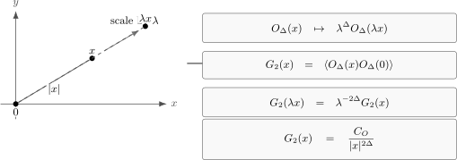
For separated scalar insertions in a translation-, rotation- and scale-invariant state, $G_2(2r)=2^{-2\Delta_O}G_2(r)$. The marked distances have the exact ratio two; the drawing illustrates the homogeneity argument, not measured correlator data.

For the critical Ising spin field,

$$\langle \sigma(x)\sigma(0)\rangle\sim {1\over |x|^{1/4}},$$

hence

$$2\Delta_\sigma={1\over4}, \qquad \Delta_\sigma={1\over8}.$$

In the language of critical phenomena one often writes the order-parameter correlator as

$$\langle \sigma(x)\sigma(0)\rangle\sim {1\over |x|^{d-2+\eta}}.$$

Comparing the two forms gives

$$\boxed{ 2\Delta_\sigma=d-2+\eta. }$$

Thus $\eta$ is simply another way of measuring the anomalous part of the scaling dimension of the order parameter. For the two-dimensional Ising model,

$$d=2, \qquad \Delta_\sigma={1\over8}, \qquad \eta={1\over4}.$$

Ising operators in the continuum

The critical Ising theory has a small set of basic fields that already explain many of the exact exponents. The spin field and the disorder field have the same scaling dimension,

$$\Delta_\sigma=\Delta_\mu={1\over8}.$$

The Majorana fermions are chiral fields with weights

$$(h_\psi,\bar h_\psi)=\left({1\over2},0\right), \qquad (h_{\bar\psi},\bar h_{\bar\psi})=\left(0,{1\over2}\right),$$

so $\Delta_\psi=\Delta_{\bar\psi}=1/2$. The energy field is the mass operator,

$$\epsilon(z,\bar z)=i\psi(z)\bar\psi(\bar z)=-2\pi u(z,\bar z)v(z,\bar z),$$

with precisely the field phases and unit normalization fixed in Lesson 11. With

$$\langle \psi(z)\psi(w)\rangle={1\over z-w}, \qquad \langle \bar\psi(\bar z)\bar\psi(\bar w)\rangle={1\over \bar z-\bar w},$$

The factor $i^2$ cancels the fermionic crossing sign, so Wick contraction gives

$$\langle \epsilon(z,\bar z)\epsilon(0,0)\rangle = {1\over z}{1\over \bar z} ={1\over |z|^2}.$$

Therefore

$$\boxed{\Delta_\epsilon=1.}$$

The fields used in the exponent calculation are summarized here; the chiral weights obey $\Delta=h+\bar h$.

Continuum field	Chiral weights $(h,\bar h)$	Scaling dimension	Physical role
Spin $\sigma$ and disorder $\mu$	$(1/16,1/16)$	$1/8$	Order and disorder observables
Energy $\epsilon=i\psi\bar\psi$	$(1/2,1/2)$	$1$	Thermal perturbation
Majorana fields $\psi$, $\bar\psi$	$(1/2,0)$, $(0,1/2)$	$1/2$	Chiral fermion correlators

The spin field $\sigma$ is not a local polynomial in $\psi$ and $\bar\psi$. It is a twist field: continuing a fermion once around a spin insertion changes its sign. This local monodromy is the continuum version of the order–disorder branch-cut construction. The energy field and spin/disorder weights are developed in Di Francesco, Mathieu and Sénéchal 1997, §§12.2.1–12.2.2, pp. 443–445.

Multi-point functions and shape data

For scaling fields $O_i$,

$$G_n(x_1,\ldots,x_n)=\langle O_1(x_1)\cdots O_n(x_n)\rangle$$

obeys the homogeneity law

$$G_n(\lambda x_1,\ldots,\lambda x_n) = \lambda^{-\sum_i \Delta_i}G_n(x_1,\ldots,x_n).$$

This is powerful, but it does not determine all multi-point functions. Translation invariance removes one vector, rotation invariance removes an overall orientation, and scale invariance removes one length. For three or more points there can still be dimensionless shape data.

For example, scale invariance alone permits a three-point function of scalar fields to be written schematically as

$$\langle O_1(x_1)O_2(x_2)O_3(x_3)\rangle = {|x_{12}|^{-\Delta_1-\Delta_2-\Delta_3}} F_{123}\left({|x_{13}|\over |x_{12}|},{|x_{23}|\over |x_{12}|}\right).$$

The two ratios determine the triangle’s shape and satisfy its triangle inequalities; its angles are not additional independent variables. Scale invariance fixes the total degree of homogeneity, but it does not fix $F_{123}$.

Full conformal invariance is stronger. For scalar primary operators it fixes the three-point function up to one coefficient:

$$\langle O_1(x_1)O_2(x_2)O_3(x_3)\rangle ={C_{123}\over |x_{12}|^{\Delta_1+\Delta_2-\Delta_3} |x_{23}|^{\Delta_2+\Delta_3-\Delta_1} |x_{31}|^{\Delta_3+\Delta_1-\Delta_2}} .$$

This separated-point formula follows from the connected conformal Ward identities; a derivation appears in Rychkov 2016, §2.2.2, preprint p. 26, PDF. The important distinction is that similarity transformations leave arbitrary triangle-shape dependence, whereas special conformal transformations remove it from scalar three-point functions. For four points, even conformal invariance leaves nontrivial functions of cross ratios. In two-dimensional complex coordinates, write the basic complex cross ratio as $\zeta$, distinct from the anomalous exponent $\eta$:

$$\zeta={z_{12}z_{34}\over z_{13}z_{24}}.$$

In the diagram, compare the two numerator pairs with the two denominator pairs. Their complex ratio is unchanged by a common Möbius transformation.

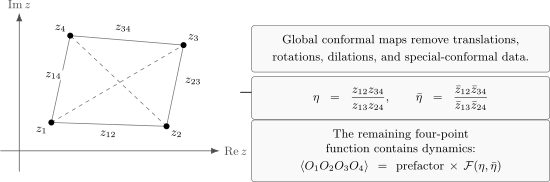
After the scalar covariance prefactor is removed, the global conformal group leaves dependence on $\zeta$ and $\bar\zeta$. The schematic point configuration distinguishes numerator and denominator pairs; the differences $z_{ij}$ are complex numbers, not only the drawn segment lengths.

The remaining function of $\zeta$ and $\bar\zeta$ contains dynamical information: operator product coefficients, exchanged scaling fields, and the consistency constraints that later become crossing symmetry. The general four-point prefactor and cross-ratio dependence are given in Rychkov 2016, §2.2.3, preprint p. 27, PDF.

Temperature as an energy perturbation

Moving the Ising model away from criticality introduces a relevant perturbation. In continuum notation,

$$S=S_*+\tau\int d^d x\,\epsilon(x)+\cdots,$$

where $\tau$ is a signed thermal scaling coupling. Its sign depends on the fixed energy-operator convention. Here $\epsilon=-2\pi uv$, whereas the Majorana action in Lesson 9 contains $-muv$. Thus in the two-dimensional Ising scaling limit,

$$m=2\pi\tau,\qquad \tau={2(K-K_c)\over\pi a} \quad\text{to leading scaling order}.$$

Consequently $\tau>0$ is the ordered side. At fixed exchange $J>0$, $K=J/T$ decreases when temperature increases, so $\tau$ has the opposite sign to $T-T_c$. This sign convention does not affect the critical exponents.

More generally, the action coefficient $\tau$ has length dimension $L^{-y_t}$ and RG eigenvalue

$$y_t=d-\Delta_\epsilon.$$

The correlation length is the scale at which the effective dimensionless perturbation becomes order one:

$$|\tau|\xi^{y_t}\sim 1.$$

Introduce the dimensionless microscopic scaling field $\hat\tau=a^{y_t}\tau$. Then

$$\boxed{ {\xi\over a}\propto |\hat\tau|^{-\nu}, \qquad \nu={1\over d-\Delta_\epsilon}. }$$

For the two-dimensional Ising model,

$$d=2, \qquad \Delta_\epsilon=1, \qquad \nu=1.$$

The relativistic Majorana excitation gap is nonnegative, while its mass parameter is signed:

$$E_{\rm gap}=|m|,\qquad \xi_\psi={1\over |m|}.$$

Here the continuum velocity is one and $\xi_\psi$ is the fermion’s exponential decay length. For a different operator $O$, the exponential length $\xi_O$ is set by the lightest state with nonzero overlap with $O$. For example, Wick contraction of the free massive energy bilinear gives a correlator proportional to

$$m^2\bigl[K_1(|m|r)^2-K_0(|m|r)^2\bigr],$$

where $K_\nu$ is a modified Bessel function. Each massive propagator comes from the scalar $K_0$ kernel and its derivative, so the bilinear has a two-particle threshold and decays as $e^{-2|m|r}$ times a power: $\xi_\epsilon=1/(2|m|)$. The Gaussian kernel and fermionic contraction are explained in Di Francesco, Mathieu and Sénéchal 1997, §§2.3.4–2.3.5, pp. 34–36. These channel-dependent amplitudes leave $\nu=1$ unchanged. In scaling estimates below, $\xi$ denotes a characteristic length proportional to $|m|^{-1}$; it is not asserted to equal every $\xi_O$.

Specific heat from the energy correlator

The singular specific heat is controlled by energy fluctuations. For $f=-V^{-1}\log Z$ and the linear thermal source above, $-\partial_\tau^2 f$ is the integrated connected energy correlator. Converting to physical temperature supplies nonuniversal factors and regular background terms; its leading singular part is therefore

$$C_{\rm sing} \sim \int d^d x\,\langle \epsilon(x)\epsilon(0)\rangle_c.$$

The connected correlator is used because the identity contribution has been subtracted. Near the fixed point,

$$\langle \epsilon(x)\epsilon(0)\rangle_c\sim {1\over |x|^{2\Delta_\epsilon}} \qquad (a\ll |x|\ll \xi).$$

Thus

$$C_{\rm sing} \sim \int_a^\xi dr\,r^{d-1-2\Delta_\epsilon}.$$

The annulus below shows the range that generates the two-dimensional logarithm. Inspect how every equal interval of $\log r$ contributes equally.

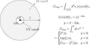
For $d=2$ and $\Delta_\epsilon=1$, the scaling-window estimate is $2\pi C_\epsilon\int_a^\xi dr/r=2\pi C_\epsilon\log(\xi/a)$. The unit-normalized field has $C_\epsilon=1$. The sharp annulus approximates the microscopic and massive crossovers; its radii are schematic, and the exact heat-capacity background is not determined by this estimate.

Writing $p=d-2\Delta_\epsilon$, the regulated radial integral gives

$$\int_a^\xi dr\,r^{p-1} \sim \begin{cases} \xi^p/p, & p>0,\\ \log(\xi/a), & p=0,\\ C_{\rm UV}-\xi^p/|p|, & p<0. \end{cases}$$

For $p<0$, the constant $C_{\rm UV}$ belongs to the cutoff-dependent analytic background. The remaining $\xi^p$ term can give a finite nonanalytic correction, such as a cusp or a singularity in a higher derivative. This is not guaranteed by the exponent alone: an even integer power with matching phase amplitudes can be analytic, and a singular amplitude can vanish. Thus UV dominance permits, but does not prove, a residual nonanalyticity.

For the two-dimensional Ising model,

$$d=2, \qquad \Delta_\epsilon=1,$$

so the energy integral is logarithmic:

$$\boxed{ C_{\rm sing}\sim \log {\xi\over a}\sim -\log |\hat\tau|. }$$

This is why the specific-heat exponent is quoted as $\alpha=0$ but the singularity is still present.

The same conclusion is consistent with hyperscaling, provided the fixed point is below its upper critical dimension and no dangerously irrelevant coupling changes the free-energy scaling. At the level of leading powers, one correlation volume contributes an order-one free energy:

$$a^d f_{\rm sing}\sim (a/\xi)^d\sim |\hat\tau|^{d\nu}, \qquad\text{up to logarithms}.$$

Logarithms cannot be discarded when differentiating at $\alpha=0$. For one two-dimensional Majorana field, the Pfaffian supplies the factor one-half. With a circular momentum cutoff $\Lambda$ and a mass-independent measure, radial integration gives

$$\begin{aligned} f(m)-f(0) &=-{1\over2}\int_{|k|<\Lambda}{d^2k\over(2\pi)^2} \log\left(1+{m^2\over k^2}\right),\\ f_{\rm sing}(m) &={m^2\over4\pi}\log{|m|\over\Lambda} \quad (|m|\ll\Lambda), \end{aligned}$$

up to terms analytic in $m^2$. The negative second thermal derivative has precisely the logarithmic divergence above. If the leading heat-capacity power is $C_{\rm sing}\sim |\hat\tau|^{-\alpha}$, then

$$\boxed{\alpha=2-d\nu.}$$

For two-dimensional Ising, $d=2$ and $\nu=1$, so $\alpha=0$. The exponent relation alone does not determine the logarithm. The critical-exponents and hyperscaling page develops the underlying RG assumptions and their failure cases.

Scaling forms away from criticality

At the fixed point, a two-point function is a pure power. Away from criticality, the correlation length can appear. Work in a clustering infinite-volume phase. On the ordered side this means selecting a pure phase, for example by taking the thermodynamic limit before $h\to0^+$ or $h\to0^-$. If $O$ has a nonzero one-point function, its massive scaling law applies to the connected correlator:

$$\boxed{ \langle O(r)O(0)\rangle_{\tau,c} ={1\over r^{2\Delta_O}} \Phi_{O,c}\left({r\over \xi}\right). }$$

For $r\ll \xi$, the scaling function tends to a constant and the critical power law is recovered. For $r\gg \xi$, the connected correlator in a massive phase decays exponentially, up to powers of $r/\xi$. When $\langle O\rangle=0$, the full and connected correlators coincide.

The following illustration separates the curvature of a critical power law from an exponential tail on the same axes. It uses declared elementary functions to show the distinction.

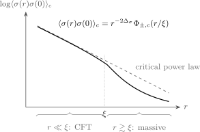
Quantitative illustration on dimensionless axes: $R=r/r_0$, $\xi/r_0=12$, and $\widetilde C=r_0^{1/4}C$. The curves are $\log\widetilde C_{\rm crit}=-\tfrac14\log R$ and $\log\widetilde C_{\rm ill}=-\tfrac14\log R-R/12$, for $1\le R\le60$. Here $r_0$ is a reference length in the scaling regime. The illustrative curve demonstrates an exponential tail; it is not the exact Ising correlator or scaling function for either phase.

For the Ising spin field, it is also useful to retain the full correlator:

$$\langle \sigma(r)\sigma(0)\rangle_\tau ={1\over r^{1/4}} \Phi_{\rm ord/dis}\left({r\over \xi}\right),$$

where $\Phi_{\rm ord}$ denotes $\tau>0$ and $\Phi_{\rm dis}$ denotes $\tau<0$ in the present convention. In the disordered phase $\Phi_{\rm dis}$ decays exponentially. In a selected ordered phase, cluster decomposition requires the full spin correlator to approach $M^2$; equivalently $\Phi_{\rm ord}(s)\sim B_{\rm ord}s^{2\Delta_\sigma}$ as $s\to\infty$. The scaling form then implies

$$a^{\Delta_\sigma}|M|\propto (a/\xi)^{\Delta_\sigma} \propto |\hat\tau|^{\nu\Delta_\sigma}.$$

Therefore the magnetization exponent is

$$\boxed{\beta_{\rm mag}=\nu\Delta_\sigma.}$$

The subscript keeps this exponent distinct from the inverse temperature often denoted by $\beta$.

Critical exponent dictionary

The two relevant Ising perturbations are the thermal field and the magnetic field:

$$S=S_*+\tau\int d^d x\,\epsilon(x)-h\int d^d x\,\sigma(x)+\cdots.$$

Their RG eigenvalues are

$$y_t=d-\Delta_\epsilon, \qquad y_h=d-\Delta_\sigma.$$

For the displayed magnetic source sign, $M=\langle\sigma\rangle=-\partial_h f$ and $\chi=\partial_hM=-\partial_h^2f\ge0$. First, the zero-field susceptibility within a clustering phase is the integrated connected spin correlator. If $d-2\Delta_\sigma>0$, its long-distance contribution dominates:

$$\chi\sim \int^{\xi}d^d x\, \langle\sigma(x)\sigma(0)\rangle_c \sim \xi^{d-2\Delta_\sigma},$$

which gives $\gamma=\nu(d-2\Delta_\sigma)$. Second, define $\hat h=a^{y_h}h$ and $\hat f=a^d f$. The leading homogeneous scaling part obeys

$$\hat f_{\rm sing}(\hat\tau,\hat h) =b^{-d}\hat f_{\rm sing}(\hat\tau b^{y_t},\hat h b^{y_h}).$$

At a thermal logarithmic resonance this relation may contain an additive analytic term; the $\hat\tau^2\log|\hat\tau|$ example above has that property. Along the critical isotherm $\hat\tau=0$ that thermal term vanishes. Choosing $b=|\hat h|^{-1/y_h}$ and differentiating with respect to the magnetic field gives

$$a^{\Delta_\sigma}|M|\propto |\hat h|^{(d-y_h)/y_h}.$$

Hence $\delta=y_h/(d-y_h)=(d-\Delta_\sigma)/\Delta_\sigma$. The sign of $M$ follows the sign of the physical field $h$.

Assuming hyperscaling and no dangerously irrelevant variable, the standard exponents are

$$\nu={1\over d-\Delta_\epsilon},$$ $$\eta=2\Delta_\sigma-d+2,$$ $$\alpha=2-d\nu,$$ $$\beta_{\rm mag}=\nu\Delta_\sigma,$$ $$\gamma=\nu(d-2\Delta_\sigma),$$

and

$$\delta={d-\Delta_\sigma\over \Delta_\sigma}.$$

For the two-dimensional Ising dimensions,

$$d=2, \qquad \Delta_\sigma={1\over8}, \qquad \Delta_\epsilon=1,$$

we obtain

$$\boxed{ \nu=1, \qquad \eta={1\over4}, \qquad \alpha=0\text{ with a logarithm}, \qquad \beta_{\rm mag}={1\over8}, \qquad \gamma={7\over4}, \qquad \delta=15. }$$

This is the operator-dimension dictionary in action. The thermodynamic exponents are not independent mysteries; they are consequences of the scaling dimensions of the relevant operators.

Summary

At a critical point, long-distance observables organize into scaling fields. Their two-point functions obey

$$\langle O(x)O(0)\rangle\sim |x|^{-2\Delta_O}.$$

For the two-dimensional Ising fixed point,

$$\Delta_\sigma=\Delta_\mu={1\over8}, \qquad \Delta_\epsilon=1, \qquad \Delta_\psi={1\over2}.$$

The energy dimension gives the correlation-length exponent and controls the specific-heat singularity. The spin dimension gives the anomalous exponent and critical isotherm; together with the thermal exponent, it also gives the magnetization and susceptibility exponents. Multi-point functions are homogeneous, but their remaining dependence on dimensionless shapes is where the operator algebra begins to appear. The next pages sharpen this by deriving conformal symmetry and then the OPE.

Common pitfalls

Scaling dimensions need not be engineering dimensions. They coincide at a suitable Gaussian fixed point, but interactions generally add anomalous dimensions and shift the powers in correlation functions.

Distinguish exponent names from scaling couplings. The exponent $\beta_{\rm mag}$ is not inverse temperature. Here $\tau$ is the signed, dimensionful thermal coupling and $\hat\tau$ its dimensionless counterpart; positive $\tau$ is ordered because of the chosen energy-field phase.

The value $\alpha=0$ does not specify the singularity by itself. In the two-dimensional Ising model the specific heat is logarithmic because the energy–energy integral is marginal.

Scale invariance fixes homogeneity, not all shape dependence. Conformal invariance is the stronger statement that fixes scalar three-point functions and reduces four-point functions to functions of conformal cross ratios.

Select a clustering phase before using massive connected decay. In a pure ordered phase, $\langle\sigma(r)\sigma(0)\rangle\to M^2$ and the connected correlator decays. In the symmetric mixture of the two ordered phases, $\langle\sigma\rangle=0$ but the pair limit remains $M^2$; subtracting that mixture’s one-point function does not remove the long-range term.

Exercises

Exercise 1: Two-point homogeneity

Let $O$ be a scalar scaling field of dimension $\Delta$ in a translation- and rotation-invariant critical theory. Show that

$$\langle O(x)O(0)\rangle={C\over |x|^{2\Delta}}.$$

Solution

Let $F(r)=\langle O(x)O(0)\rangle$, where $r=|x|$. Scale covariance gives

$$F(\lambda r)=\lambda^{-2\Delta}F(r).$$

Set $r=1$ and choose $\lambda=r$. Then

$$F(r)=F(\lambda\cdot 1)=\lambda^{-2\Delta}F(1)=C r^{-2\Delta}.$$

Thus

$$F(r)={C\over r^{2\Delta}}.$$

Exercise 2: Energy fluctuations and specific heat

Use the energy correlator

$$\langle \epsilon(x)\epsilon(0)\rangle_c\sim {|x|}^{-2\Delta_\epsilon}$$

to determine the singular scaling of

$$C_{\rm sing}\sim \int_a^\xi dr\,r^{d-1-2\Delta_\epsilon}.$$

Apply the result to the two-dimensional Ising model.

Solution

If $d-2\Delta_\epsilon\ne0$, then

$$\int_a^\xi dr\,r^{d-1-2\Delta_\epsilon} ={\xi^{d-2\Delta_\epsilon}-a^{d-2\Delta_\epsilon}\over d-2\Delta_\epsilon}.$$

For $d>2\Delta_\epsilon$, the $\xi$ term dominates. For $d<2\Delta_\epsilon$, the first term vanishes as $\xi\to\infty$ while the cutoff term contributes to the analytic background. The remaining power $\xi^{d-2\Delta_\epsilon}$ can produce a finite cusp or a singularity in a higher derivative, but need not be nonanalytic: its exponent and phase amplitudes must be checked. For $d=2\Delta_\epsilon$,

$$\int_a^\xi {dr\over r}=\log(\xi/a).$$

In the two-dimensional Ising model, $d=2$ and $\Delta_\epsilon=1$, so

$$C_{\rm sing}\sim \log(\xi/a)\sim -\log |\hat\tau|.$$

Exercise 3: The two-dimensional Ising exponent dictionary

Using $d=2$, $\Delta_\sigma=1/8$, and $\Delta_\epsilon=1$, compute $\nu$, $\eta$, $\alpha$, $\beta_{\rm mag}$, $\gamma$, and $\delta$.

Solution

The correlation-length exponent is

$$\nu={1\over d-\Delta_\epsilon}={1\over2-1}=1.$$

The anomalous-dimension exponent is

$$\eta=2\Delta_\sigma-d+2={1\over4}.$$

The specific-heat exponent is

$$\alpha=2-d\nu=2-2=0,$$

with a logarithmic singularity. The magnetization exponent is

$$\beta_{\rm mag}=\nu\Delta_\sigma={1\over8}.$$

The susceptibility exponent is

$$\gamma=\nu(d-2\Delta_\sigma)=2-{1\over4}={7\over4}.$$

Finally,

$$\delta={d-\Delta_\sigma\over \Delta_\sigma} ={2-1/8\over 1/8}=15.$$

Exercise 4: Energy dimension from Majorana fields

Assume

$$\langle \psi(z)\psi(0)\rangle={1\over z}, \qquad \langle \bar\psi(\bar z)\bar\psi(0)\rangle={1\over \bar z}.$$

If $\epsilon\sim i\psi\bar\psi$, show that $\Delta_\epsilon=1$.

Solution

Wick contraction gives

$$\langle \epsilon(z,\bar z)\epsilon(0,0)\rangle \propto \langle \psi(z)\psi(0)\rangle \langle \bar\psi(\bar z)\bar\psi(0)\rangle ={1\over z\bar z} ={1\over |z|^2}.$$

A scalar operator with dimension $\Delta$ has two-point function $|z|^{-2\Delta}$. Therefore $2\Delta_\epsilon=2$, and

$$\Delta_\epsilon=1.$$

References

• P. Di Francesco, P. Mathieu, and D. Sénéchal, Conformal Field Theory. Graduate Texts in Contemporary Physics, Springer, New York (1997). DOI: 10.1007/978-1-4612-2256-9.
• S. Rychkov, EPFL Lectures on Conformal Field Theory in D ≥ 3 Dimensions (2016), arXiv:1601.05000v2. Stable preprint; Open PDF. Page locators above refer to this preprint version.

Further reading

• J. Cardy, Scaling and Renormalization in Statistical Physics. Cambridge Lecture Notes in Physics 5, Cambridge University Press (1996). DOI: 10.1017/CBO9781316036440. A compact route from scaling hypotheses to critical exponents.
• B. M. McCoy and T. T. Wu, The Two-Dimensional Ising Model. Harvard University Press, Cambridge, MA (1973). DOI: 10.4159/harvard.9780674180758. The exact lattice solution and correlation-function results.