Bosonization and Sine-Gordon–Thirring Duality

The previous page ended with a clue: neutral fermion correlators in two dimensions have the same algebraic structure as correlators of exponentials of a free scalar field. This is not an accident, and it is not merely a trick for computing determinants. In two spacetime dimensions, the operator algebra of a massless Dirac fermion can be represented by the operator algebra of a compact scalar. This is bosonization.

A fermion field, which anticommutes and has spin $1/2$, can be represented by exponentials of bosonic fields when zero modes, branch cuts, and Klein factors are included. A four-fermion current interaction changes the scalar stiffness, and a fermion mass becomes a cosine perturbation. The equivalence below uses a specified renormalized current and mass-operator prescription; the neutral operator comparison and the extension to charged soliton sectors are separate steps.

This page develops the dictionary in the normalization closest to the preceding two-dimensional notes. The goal is not to prove every global subtlety of bosonization on an arbitrary Riemann surface. The goal is to make the local operator identities and the sine-Gordon–Thirring map usable.

Required background. The Schwinger model and gauge-invariant correlators supplies the neutral fermion determinant that becomes a bosonic vertex-operator correlator. Helpful background. Gauge fields in two dimensions supplies the chiral propagators and complex-coordinate conventions.

Fermion determinants as boson correlators

Two-dimensional bosonization conventions. We use Euclidean complex coordinates

$$z=x^1+i x^2, \qquad \bar z=x^1-i x^2.$$

With $x^2=\tau$ and $t=-i\tau$, their boundary values are $z=-x^-$ and $\bar z=x^+$; field phases and the $i0$ prescription continue together as in the preceding chiral-propagator lesson. We use two independent chiral bosons and define the relative, sine-Gordon combination by

$$\Phi(z,\bar z)=\phi_R(z)-\phi_L(\bar z),$$

with two-point functions

$$\langle \phi_R(z)\phi_R(w)\rangle=-\log{z-w\over a}, \qquad \langle \phi_L(\bar z)\phi_L(\bar w)\rangle=-\log{\bar z-\bar w\over a},$$

and

$$\langle \phi_R(z)\phi_L(\bar w)\rangle=0.$$

The short-distance length $a$ is a UV cutoff. With this convention,

$$\langle \Phi(z,\bar z)\Phi(w,\bar w)\rangle =-\log{|z-w|^2\over a^2}.$$

The sum $\widetilde\Phi=\phi_R+\phi_L$ is the dual combination. Which of $\Phi$ and $\widetilde\Phi$ is called “the boson” varies across the literature. Keeping the relative combination explicit prevents a sign mismatch between the fermion mass operator and the topological current.

Normal ordering $: \cdots :$ is defined with respect to this free scalar. Overall constants in vertex operators depend on the cutoff convention and are absorbed into normalization constants.

Relation to canonical scalar normalization. The chiral convention above corresponds to the nonchiral free-boson action

$$S={1\over8\pi}\int d^2x\,(\partial_\mu\Phi)^2,$$

for which $:e^{i\phi_R}:$ has holomorphic weight $1/2$ and can represent a chiral fermion. If instead one uses the canonical normalization

$$S={1\over2}\int d^2x\,(\partial_\mu\varphi_0)^2,$$

then

$$\Phi=\sqrt{4\pi}\,\varphi_0.$$

In that convention the free-fermion mass operator corresponds to a sine-Gordon cosine with $\beta_{\mathrm{SG}}^2=4\pi$. Many apparent disagreements in bosonization formulas are only this rescaling.

As in the preceding two lessons, use capital $\Psi_{R,L}$ for the CFT-normalized chiral fields and lowercase $\psi_{R,L}$ for action-normalized fermions:

$$\Psi_{R,L}=\sqrt{2\pi}\,\psi_{R,L}, \qquad \langle\Psi_R(z)\Psi_R^\dagger(w)\rangle =2\pi\langle\psi_R(z)\psi_R^\dagger(w)\rangle.$$

The CFT-normalized propagator is

$$\langle \Psi_R(z)\Psi_R^\dagger(w)\rangle={1\over z-w}.$$

Wick’s theorem gives the $n$-particle neutral correlator

$$\left\langle \Psi_R(z_1)\cdots\Psi_R(z_n) \Psi_R^\dagger(w_1)\cdots\Psi_R^\dagger(w_n) \right\rangle =(-1)^{n(n-1)/2}\det_{1\le i,j\le n}{1\over z_i-w_j}.$$

Reversing the displayed ascending order of the $n$ dagger fields requires $n(n-1)/2$ fermion interchanges; the reversed order gives the determinant without the prefactor. For the order actually printed, the four-point function is exchange minus direct:

$$\langle\Psi_R(z_1)\Psi_R(z_2) \Psi_R^\dagger(w_1)\Psi_R^\dagger(w_2)\rangle ={1\over(z_1-w_2)(z_2-w_1)} -{1\over(z_1-w_1)(z_2-w_2)}.$$

The separate Cauchy determinant identity is

$$\boxed{ \det_{i,j}{1\over z_i-w_j} ={ \prod_{i<j}(z_i-z_j)\prod_{i<j}(w_j-w_i) \over \prod_{i,j}(z_i-w_j) }. }$$

This determinant is direct minus exchange when $n=2$; its relation to a fermion correlator still requires the declared operator order.

Now compare this with a Gaussian scalar. For vertex operators

$$V_\alpha(z)=:e^{i\alpha\phi_R(z)}:,$$

Wick’s theorem gives

$$\left\langle \prod_k V_{\alpha_k}(z_k)\right\rangle =\begin{cases} \displaystyle \prod_{i<j}\left({z_i-z_j\over a}\right)^{\alpha_i\alpha_j}, & \sum_k\alpha_k=0,\\[1.3em] 0, & \sum_k\alpha_k\ne 0, \end{cases}$$

where the second line uses the invariant zero-mode vacuum and allowed charges of the chosen compactification. Continuous charges can also be used in the formal noncompact Gaussian calculation, with its zero-mode integral understood distributionally. Taking charges $+1$ at the $z_i$ and charges $-1$ at the $w_j$ gives

$$\left\langle \prod_{i=1}^n :e^{i\phi_R(z_i)}: \prod_{j=1}^n :e^{-i\phi_R(w_j)}: \right\rangle =a^n{ \prod_{i<j}(z_i-z_j) \prod_{i<j}(w_i-w_j) \over \prod_{i,j}(z_i-w_j) }$$

with the same insertion order and analytic branches throughout. Since $\prod_{i<j}(w_i-w_j)=(-1)^{n(n-1)/2}\prod_{i<j}(w_j-w_i)$, the relation for the printed ascending dagger order is exactly

$$\begin{aligned} &\left\langle\prod_{i=1}^n\Psi_R(z_i) \prod_{j=1}^n\Psi_R^\dagger(w_j)\right\rangle\\ &\quad=a^{-n} \left\langle\prod_{i=1}^n V_{+1}(z_i) \prod_{j=1}^n V_{-1}(w_j)\right\rangle =(-1)^{n(n-1)/2}\det C, \qquad C_{ij}={1\over z_i-w_j}. \end{aligned}$$

The raw vertex product carries $a^n$. Each of the $2n$ fermion prefactors contributes $a^{-1/2}$, so this cutoff factor cancels. The next diagram keeps both the ordering sign and this normalization visible.

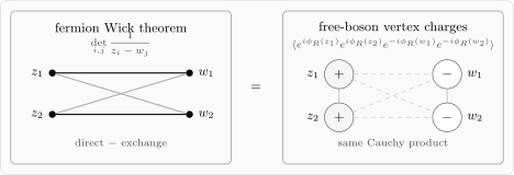
For the printed ascending dagger order, the $n=2$ fermion correlator is exchange minus direct, or minus the Cauchy determinant. It equals $a^{-2}$ times the displayed raw cutoff-normal-ordered vertex correlator. Charges and insertion order are held fixed; the contraction lines are schematic.

Thus the local identification

$$\boxed{ \Psi_R(z)\sim {F_R\over\sqrt a}:e^{i\phi_R(z)}:, \qquad \Psi_R^\dagger(z)\sim {F_R^\dagger\over\sqrt a}:e^{-i\phi_R(z)}: }$$

reproduces all neutral right-moving correlators. Similarly,

$$\boxed{ \Psi_L(\bar z)\sim {F_L\over\sqrt a}:e^{i\phi_L(\bar z)}:, \qquad \Psi_L^\dagger(\bar z)\sim {F_L^\dagger\over\sqrt a}:e^{-i\phi_L(\bar z)}:. }$$

These are the CFT prefactors. For canonical fermions,

$$\psi_{R,L}={\Psi_{R,L}\over\sqrt{2\pi}} \sim {F_{R,L}\over\sqrt{2\pi a}}:e^{i\phi_{R,L}}:.$$

Likewise $J_R=:\!\Psi_R^\dagger\Psi_R\!:=2\pi j_R$, so a physical source couples to $J_R/(2\pi)$, not to an unrescaled unit-OPE current. The Lorentzian Dirac Lagrangians below use canonical lowercase $\psi$ and the physical current.

The factors $F_R,F_L$ are Klein factors. They commute with the bosonic oscillators but anticommute among themselves, ensuring

$$\{\Psi_R,\Psi_L\}=0.$$

For many local correlation functions with equal numbers of each species, the Klein factors only provide the overall fermionic sign. For operator algebra, Hilbert-space construction, boundary conditions, or finite-size systems, they are not optional.

The determinant formula assumes a complex chiral fermion. For a real Majorana fermion, Wick’s theorem instead gives a Pfaffian of the antisymmetric matrix of two-point functions. Two Majorana fields combine into one Dirac field, which is why the charged Cauchy-determinant form is the most direct doorway to bosonization.

What the symbol “$\sim$” means

The formula $\Psi_R\sim F_R:e^{i\phi_R}:$ is an operator dictionary inside correlation functions with a specified normalization and spin structure. It is not an equality of ordinary commuting classical fields. The exponential carries the correct local singularities; the Klein factor carries the global anticommutation data.

Scaling dimensions and the neutrality condition

The same Gaussian calculation immediately gives the scaling dimension of a vertex operator. For a chiral operator,

$$\langle V_\alpha(z)V_{-\alpha}(w)\rangle =\left({a\over z-w}\right)^{\alpha^2}.$$

A holomorphic primary field of weight $h$ has two-point function proportional to $(z-w)^{-2h}$, so

$$\boxed{h[V_\alpha]={\alpha^2\over2}.}$$

The fermion operator corresponds to $\alpha=1$ and therefore has $h=1/2$, as it should.

For the nonchiral vertex operator

$$V_{\alpha,\bar\alpha}(z,\bar z) =:e^{i\alpha\phi_R(z)+i\bar\alpha\phi_L(\bar z)}:,$$

we have

$$h={\alpha^2\over2}, \qquad \bar h={\bar\alpha^2\over2},$$

so the scaling dimension and Euclidean spin are

$$\Delta=h+\bar h={\alpha^2+\bar\alpha^2\over2}, \qquad s=h-\bar h={\alpha^2-\bar\alpha^2\over2}.$$

A right-moving spinor has spin $+1/2$, so any bosonic representation of an interacting right-moving fermion must satisfy

$$\boxed{\alpha^2-\bar\alpha^2=1.}$$

This simple equation is the seed of anomalous fermion dimensions in the massless Thirring model.

The neutrality condition is just as important. The nonchiral correlator

$$\left\langle\prod_k :e^{i\alpha_k\Phi(x_k)}:\right\rangle$$

contains the zero mode of $\Phi$. Since the free boson action depends only on derivatives, the constant mode is integrated over. The integral

$$\int d\Phi_0\,\exp\left(i\Phi_0\sum_k\alpha_k\right)$$

vanishes unless

$$\boxed{\sum_k\alpha_k=0.}$$

Equivalently, if one regulates the theory in a box of size $R$, nonneutral correlators carry powers of $R$ and disappear in the infinite-volume limit after normalizing the vacuum. This is the infrared counterpart of charge conservation.

The vertex-operator OPE

The operator product expansion of vertex operators follows from separating the contraction between nearby points from the normal-ordered product:

$$:e^{i\alpha\phi_R(z)}::e^{i\beta\phi_R(w)}: =\exp\left[-\alpha\beta\langle\phi_R(z)\phi_R(w)\rangle\right] :e^{i\alpha\phi_R(z)+i\beta\phi_R(w)}:.$$

Using

$$\langle\phi_R(z)\phi_R(w)\rangle=-\log{z-w\over a},$$

and expanding the slowly varying field $\phi_R(z)$ around $w$, we get

$$\boxed{ :e^{i\alpha\phi_R(z)}::e^{i\beta\phi_R(w)}: \sim \left({z-w\over a}\right)^{\alpha\beta} :e^{i(\alpha+\beta)\phi_R(w)}: \left[1+i\alpha(z-w)\partial\phi_R(w)+\cdots\right]. }$$

For $\alpha=1$ and $\beta=-1$,

$$:e^{i\phi_R(z)}::e^{-i\phi_R(w)}: \sim {a\over z-w}\left[1+i(z-w)\partial\phi_R(w)+\cdots\right],$$

which reproduces the fermion short-distance singularity. For $\alpha=\beta=1$,

$$:e^{i\phi_R(z)}::e^{i\phi_R(w)}: \sim {z-w\over a}:e^{2i\phi_R(w)}: +\cdots.$$

The zero as $z\to w$ is the bosonic representation of Pauli exclusion for two identical chiral fermions. The anticommutation sign is encoded by the branch choice and Klein factors; the vanishing of the local product is already visible in the OPE.

The following fusion diagram keeps the separation-to-cutoff ratio explicit.

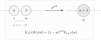
When two cutoff-normal-ordered vertex operators approach each other, their charges add. The singular or vanishing dimensionless prefactor is $[(z-w)/a]^{\alpha\beta}$. This is a schematic fusion rule at fixed cutoff normalization.

This OPE is the local engine behind bosonization. The global theory contains more data: compactification radius, allowed charges, spin structures, and Klein factors. But the short-distance algebra already knows why exponentials of a free scalar can behave like fermions.

Current dictionary and charge normalization

After continuation to Lorentzian coordinates $(x^0,x^1)=(t,x)$, use

$$\eta_{\mu\nu}=\operatorname{diag}(+,-), \qquad \epsilon^{01}=+1, \qquad \epsilon_{01}=-1.$$

This orientation fixes the vector current as the derivative of the relative boson. In the chiral normalization used above,

$$j^\mu={1\over2\pi}\epsilon^{\mu\nu}\partial_\nu\Phi.$$

Equivalently, at the free-fermion point $\Phi=\sqrt{4\pi}\,\varphi_0$,

$$j^\mu={1\over\sqrt\pi}\epsilon^{\mu\nu}\partial_\nu\varphi_0.$$

The charge is therefore a winding number:

$$Q=\int dx\,j^0={1\over2\pi}\left[\Phi(+\infty)-\Phi(-\infty)\right] ={1\over\sqrt\pi}\left[\varphi_0(+\infty)-\varphi_0(-\infty)\right].$$

At nonzero Thirring coupling the canonically normalized sine-Gordon field has a coupling-dependent radius, and the corresponding dictionary becomes $j^\mu=(\beta_{\mathrm{SG}}/2\pi)\epsilon^{\mu\nu}\partial_\nu\varphi$. The free point $\beta_{\mathrm{SG}}^2=4\pi$ reproduces the coefficient $1/\sqrt\pi$.

Here $j^\mu$ is the renormalized current, not an undefined coincident product. We use Coleman’s Ward-identity normalization and the corresponding finite definition of the current interaction; a different prescription can redefine the parameter called $g_{\mathrm{Th}}$. In Coleman 1975, §I, pp.2088–2089, Eqs.(1.4)–(1.10), §IV, p.2093, Eqs.(4.25)–(4.29), and notation note1, p.2096, the current has unit fermion-number charge. His notation sets $\epsilon_{01}=+1$, so his $\epsilon^{01}=-1$: his displayed minus dual-current formula gives precisely the positive coefficient used here. The scalar need not be reversed.

This current relates the local dictionary to the soliton interpretation. A charged fermion operator changes the winding sector; that extension is more than equality of neutral correlators.

The massless Thirring model as a free boson with a shifted radius

The massless Thirring model uses the action-normalized Dirac field and the renormalized current just specified:

$$\mathcal L_{\mathrm{Th},0} =\bar\psi i\gamma^\mu\partial_\mu\psi -{g_{\mathrm{Th}}\over2}j_\mu j^\mu, \qquad j^\mu=[\bar\psi\gamma^\mu\psi]_{\mathrm{ren}}.$$

The interaction is classically marginal: $[\psi]=1/2$, so the current has dimension $1$ and $j_\mu j^\mu$ has dimension $2$. With the matched current-product prescription, its bosonic image can be derived directly. The fixed compact phase has $j^\mu=\epsilon^{\mu\nu}\partial_\nu\Phi/(2\pi)$, hence

$$j_\mu j^\mu ={(\partial_x\Phi)^2-(\partial_t\Phi)^2\over4\pi^2} =-{1\over4\pi^2}(\partial_\mu\Phi)^2.$$

Adding the interaction to the free kinetic term therefore gives

$$\mathcal L_{\mathrm{bos},0} ={K\over8\pi}(\partial_\mu\Phi)^2, \qquad K=1+{g_{\mathrm{Th}}\over\pi}.$$

The products on both sides have the same subtraction prescription; this is not multiplication of unsmeared distributions at coincident points. A positive Gaussian Hamiltonian requires $K>0$, or $g_{\mathrm{Th}}>-\pi$. Define the interacting canonical field and its cosine coupling by

$$\varphi={\sqrt K\over\sqrt{4\pi}}\,\Phi, \qquad \beta_{\mathrm{SG}}=\sqrt{4\pi\over K}>0.$$

Then

$$\mathcal L_{\mathrm{bos},0}={1\over2}(\partial\varphi)^2, \qquad \Phi=\beta_{\mathrm{SG}}\varphi, \qquad j^\mu={\beta_{\mathrm{SG}}\over2\pi} \epsilon^{\mu\nu}\partial_\nu\varphi.$$

The compact phase still has period $2\pi$; the canonical field’s period is $2\pi/\beta_{\mathrm{SG}}$. Thus the current interaction changes the radius measured with a canonical kinetic term. The result is the Coleman relation

$$\boxed{ {4\pi\over\beta_{\mathrm{SG}}^2} =1+{g_{\mathrm{Th}}\over\pi}. }$$

This agrees with Coleman 1975, §IV, p.2093, Eqs.(4.22)–(4.29). The positive-kinetic condition concerns the massless theory; it is not by itself a continuum-existence argument for every cosine perturbation.

To display the fermion exponents, introduce normalized interacting chiral fields $\chi_R,\chi_L$ with contractions $-\log[(z-w)/a]$ and $-\log[(\bar z-\bar w)/a]$, respectively, and

$$\chi_R-\chi_L=\sqrt{4\pi}\,\varphi=\sqrt K\,\Phi.$$

These coincide with the original free-point fields $\phi_R,\phi_L$ when $K=1$; at other couplings they must not be substituted for the fixed compact phase without the factor $\sqrt K$. The interacting fermions have the form

$$\psi_R\sim F_R:e^{iu\chi_R+iv\chi_L}:, \qquad \psi_L\sim F_L:e^{iv\chi_R+iu\chi_L}:,$$

with cutoff-dependent operator normalizations understood, and

$$u={\sqrt K+1/\sqrt K\over2}, \qquad v={\sqrt K-1/\sqrt K\over2}.$$

We reserve $a$ for the cutoff length. These dimensionless exponents obey

$$u^2-v^2=1, \qquad \lambda\equiv u-v={1\over\sqrt K}, \qquad u+v=\sqrt K.$$

The first condition keeps spin $1/2$, while the second makes the mass bilinear’s exponent $\lambda(\chi_R-\chi_L)=\Phi$. Consequently

$$\langle\psi_R(z,\bar z)\psi_R^\dagger(0,0)\rangle \propto {1\over z^{u^2}\bar z^{v^2}} ={1\over z}\,{1\over |z|^{2v^2}}, \qquad \Delta_\psi={K+K^{-1}\over4}.$$

The first factor gives the spinor transformation law; the second is an anomalous power. Its real-time boundary value uses the right-moving $x^-$ pole and the same time-ordered branch as lesson23, not an unsigned power of a Lorentzian squared distance. At $g_{\mathrm{Th}}=0$, $u=1$, $v=0$, $\Delta_\psi=1/2$, and $\beta_{\mathrm{SG}}^2=4\pi$.

Adding a mass: the cosine perturbation

With the Lorentzian Dirac convention used earlier in the course, the massive Thirring model adds

$$\Delta\mathcal L_M=-m\bar\psi\psi.$$

In chiral components,

$$\bar\psi\psi=\psi_L^\dagger\psi_R+\psi_R^\dagger\psi_L.$$

Using the interacting-fermion representation,

$$\psi_L^\dagger\psi_R \sim :e^{i(u-v)(\chi_R-\chi_L)}:.$$

The normalized interacting chiral fields give

$$\lambda=u-v={1\over\sqrt K}, \qquad \lambda(\chi_R-\chi_L)=\Phi=\beta_{\mathrm{SG}}\varphi.$$

Fix the relative Klein-factor phase and define the positive cutoff-dependent normalization $C_m>0$ so that the mass operator becomes

$$\boxed{ \bar\psi\psi\ \longleftrightarrow\ -C_m\cos\Phi, }$$

Under Wick rotation, the fermion mass contribution is

$$S_{E,m}=+m\int d^2x\,\bar\psi\psi \ \longleftrightarrow\ -mC_m\int d^2x\,\cos\Phi.$$

The additive vacuum energy can be chosen independently. The negative cosine coefficient is conventionally written as a positive coefficient multiplying $1-\cos\Phi$ in a fixed cutoff parametrization; any normal-ordering factor is absorbed into that coefficient. The resulting sine-Gordon action is

$$\boxed{ S_{\mathrm{SG},E} =\int d^2x\left[ {1\over2}(\partial_\mu\varphi)^2 +{\mu\over\beta_{\mathrm{SG}}^2}\left(1-\cos(\beta_{\mathrm{SG}}\varphi)\right) \right] }$$

in canonical normalization, or equivalently to

$$S_E={K\over8\pi}\int d^2x\,(\partial_\mu\Phi)^2 +\widetilde\mu\int d^2x\,[1-\cos\Phi]$$

in the fixed compact-phase normalization, with $\beta_{\mathrm{SG}}=\sqrt{4\pi}\lambda$. The displayed cosine is a cutoff-normal-ordered composite operator; its normalization is included in its coefficient. For $m>0$, the chosen convention has $\mu>0$ and $\widetilde\mu>0$. Their precise magnitudes relative to $m$ and the cutoff are nonuniversal; the sign map above, the operator algebra, and the dimensionless coupling $\beta_{\mathrm{SG}}$ are fixed once the renormalization convention and Klein-factor phase are chosen.

The next map separates canonical rescaling from the optional mass perturbation.

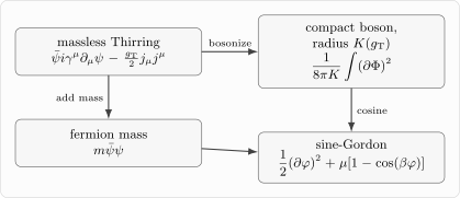
With the compact phase held fixed, the current interaction gives stiffness $K=1+g_{\mathrm{Th}}/\pi>0$. Canonical rescaling changes its radius and gives the exponents $u,v$. With $\mathcal L_{M,m}=-m\bar\psi\psi$, $S_{E,m}=+m\int\bar\psi\psi$, and $\bar\psi\psi=-C_m\cos(\beta\varphi)$, the positive-mass Euclidean potential is proportional to $1-\cos(\beta\varphi)$.

At matched current and mass-composite prescriptions, the neutral mass-perturbation expansions agree. Coleman establishes this comparison with an infrared switching function and does not identify it with a complete constructive-existence proof; see Coleman 1975, §I, p.2089, and §IV, pp.2092–2093. The relation is strong–weak in an important sense. From

$${4\pi\over \beta_{\mathrm{SG}}^2}=1+{g_{\mathrm{Th}}\over\pi},$$

large positive Thirring coupling corresponds to small sine-Gordon coupling. In that regime the sine-Gordon semiclassical soliton is a useful description of the fermionic excitation.

Scaling dimension of the cosine

The mass perturbation also provides a direct consistency check. Because

$$\left\langle :e^{i\Phi(x)}: :e^{-i\Phi(0)}: \right\rangle \propto {1\over |x|^{2\lambda^2}},$$

the cosine has scaling dimension

$$\boxed{ \Delta_{\cos}=\lambda^2 ={\beta_{\mathrm{SG}}^2\over4\pi} ={1\over1+g_{\mathrm{Th}}/\pi}. }$$

At the free-fermion point, $\Delta_{\cos}=1$, the dimension of $\bar\psi\psi$. About the massless Gaussian fixed point the cosine is relevant for $\beta_{\mathrm{SG}}^2<8\pi$, marginal to first order at $8\pi$, and irrelevant for $\beta_{\mathrm{SG}}^2>8\pi$. The relevant interval corresponds to $g_{\mathrm{Th}}>-\pi/2$, a stronger condition than positivity of the massless kinetic term.

A finite-cutoff Hamiltonian with positive kinetic energy and a bounded cosine potential can be defined beyond that interval. This does not establish the same interacting continuum limit: the normal-ordered continuum Hamiltonian considered by Coleman is unbounded below for $\beta_{\mathrm{SG}}^2>8\pi$ (Coleman 1975, §III, p.2091, Eqs.(3.6)–(3.7), and §V.A, pp.2093–2094). At the marginal point further running matters. We use the regulated operator dictionary and the relevant cosine regime here; neither the dimension formula nor the schematic action is a proof of a continuum massive equivalence at arbitrary coupling.

Solitons as fermions

The sine-Gordon potential is periodic. Its classical vacua are

$$\beta_{\mathrm{SG}}\varphi=2\pi n, \qquad n\in\mathbb Z.$$

A finite-energy static configuration must approach vacua at spatial infinity:

$$\varphi(x\to-\infty)={2\pi n_-\over\beta_{\mathrm{SG}}}, \qquad \varphi(x\to+\infty)={2\pi n_+\over\beta_{\mathrm{SG}}}.$$

The integer

$$Q_{\mathrm{top}}=n_+-n_- ={\beta_{\mathrm{SG}}\over2\pi}\left[\varphi(+\infty)-\varphi(-\infty)\right]$$

is the soliton number. The one-soliton solution for the potential

$$V(\varphi)={m_{\mathrm{SG}}^2\over\beta_{\mathrm{SG}}^2} \left(1-\cos\beta_{\mathrm{SG}}\varphi\right)$$

is

$$\boxed{ \varphi_{\mathrm{sol}}(x-X) ={4\over\beta_{\mathrm{SG}}}\arctan e^{m_{\mathrm{SG}}(x-X)}. }$$

It interpolates from $0$ to $2\pi/\beta_{\mathrm{SG}}$. For a static finite-energy solution, the first integral of the field equation is

$${1\over2}\left({d\varphi\over dx}\right)^2 =V(\varphi),$$

where the integration constant vanishes because both terms go to zero in a vacuum. The energy can therefore be evaluated without inserting the detailed profile:

$$M_{\mathrm{sol}} =\int_0^{2\pi/\beta_{\mathrm{SG}}} d\varphi\,\sqrt{2V(\varphi)}.$$

Evaluating the elementary integral gives

$$\boxed{ M_{\mathrm{sol}}={8m_{\mathrm{SG}}\over\beta_{\mathrm{SG}}^2}. }$$

The interacting bosonized current,

$$j^\mu={\beta_{\mathrm{SG}}\over2\pi} \epsilon^{\mu\nu}\partial_\nu\varphi,$$

identifies fermion number with topological charge:

$$Q_F=\int dx\,j^0 ={\beta_{\mathrm{SG}}\over2\pi}\left[\varphi(+\infty)-\varphi(-\infty)\right] =Q_{\mathrm{top}}.$$

Thus the elementary fermion of the Thirring description is represented, in the sine-Gordon description, by a soliton. The antifermion is the antisoliton.

Topological charge alone does not prove fermionic statistics. A useful way to see the missing ingredient is to write a charge-raising string using the canonical momentum $\Pi=\dot\varphi$:

$$\mathcal S^\dagger(x)\ \propto\ :\exp\left[ -{2\pi i\over\beta_{\mathrm{SG}}}\int_x^\infty dy\,\Pi(y) +{i\beta_{\mathrm{SG}}\over2}\varphi(x) \right]:.$$

The half-line integral has a specified infrared and endpoint prescription. From $[\varphi(y),\Pi(z)]=i\delta(y-z)$, its first term gives $[\varphi(y),\mathcal S^\dagger(x)]=(2\pi/\beta_{\mathrm{SG}})\Theta(y-x)\mathcal S^\dagger(x)$, so $[Q_F,\mathcal S^\dagger]=\mathcal S^\dagger$. For distinct $x,y$, the commutator of the two exponents is $i\pi\,\operatorname{sgn}(x-y)$; the Baker–Campbell–Hausdorff exchange factor is therefore $-1$. The local phase matters: the string alone would commute with another such string. Contact normalization and the second fermion component require the corresponding regulator and Klein-factor choices.

This is the mechanism in Mandelstam 1975, §II, p.3027, Eqs.(2.4)–(2.8), and §§III–IV, pp.3028–3029: nonlocal bosonic operators supply charged fermionic sectors and satisfy the renormalized Thirring equations. His coupling relation is $g_{\mathrm M}/\pi=1-4\pi/\beta_{\mathrm{SG}}^2$, so $g_{\mathrm M}=-g_{\mathrm{Th}}$ when comparing the displayed parameter formulas. His point-split conserved current, rather than the naive unrenormalized bilinear, is essential. Our string uses the opposite half-line convention from his displayed construction and fixes its charge directly by the commutator above.

These operator statements do not turn every classical profile into an exact one-particle quantum state. The mass $8m_{\mathrm{SG}}/\beta_{\mathrm{SG}}^2$ is classical; quantum masses and particle stability require the specified interacting theory and coupling regime.

The two panels below compare an explicitly prescribed force with the untilted classical kink.

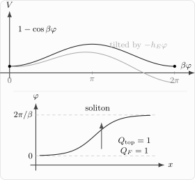
In the untilted classical potential, neighboring minima differ by $2\pi/\beta$ and an increasing kink carries unit fermion number. The upper panel compares $\mathcal V(\theta)=1-\cos\theta$ with prescribed forcing $\mathcal V(\theta)-\eta\theta$ at $\eta=1/5$, where $\theta=\beta\varphi$ and $\mathcal V=\beta^2V/m_{\mathrm{SG}}^2$. The lower panel uses the exact classical kink $\theta(X)=4\arctan e^X$, $X=m_{\mathrm{SG}}(x-X_0)$. These dimensionless classical examples do not describe a dynamical theta-vacuum potential or a quantum pair-production rate.

The comparison explains why a local fermion in one description becomes a winding-changing operator in the other. Extending the neutral operator correspondence to a Hilbert-space statement requires matching charged sectors, compactification and boundary conditions; the elementary Gaussian identity alone does not establish those global identifications.

Tilted vacua and the electric-field interpretation

First take $A_\mu$ to be a prescribed external field coupled through $D_\mu=\partial_\mu-iqA_\mu$. The interaction is $+qA_\mu j^\mu$. With $E=F_{01}$, integration by parts gives

$$\begin{aligned} qA_\mu j^\mu &={q\beta_{\mathrm{SG}}\over2\pi} \left(A_0\partial_x\varphi-A_1\partial_t\varphi\right)\\ &={q\beta_{\mathrm{SG}}\over2\pi}E\varphi +\text{total derivative}. \end{aligned}$$

For a uniform fixed $E$, the static potential is therefore

$$V(\varphi) ={m_{\mathrm{SG}}^2\over\beta_{\mathrm{SG}}^2} \left(1-\cos\beta_{\mathrm{SG}}\varphi\right) -h_E\varphi, \qquad h_E={qE\beta_{\mathrm{SG}}\over2\pi}.$$

This fixes the sign and normalization in the site’s charge convention. Under $\varphi\mapsto\varphi+2\pi/\beta_{\mathrm{SG}}$, the potential density changes by $-qE$. With $\theta=\beta_{\mathrm{SG}}\varphi$ and $\eta=h_E\beta_{\mathrm{SG}}/m_{\mathrm{SG}}^2$, its extrema satisfy $\sin\theta=\eta$. At $0<\eta<1$, each minimum shifts to $\theta=\arcsin\eta+2\pi n$ and adjacent minima differ in energy density by $-2\pi\eta$ in the dimensionless potential. At $|\eta|>1$ no local extrema remain; the limiting $|\eta|=1$ has merged stationary points.

The uniform force assigns energies to the unwrapped winding branches; it is not a single-valued periodic potential on the compact angle. The surviving wells are local, not global minima. The field is held fixed in this forcing problem. A kink–antikink pair can enclose a region in a different well and receive work from the external source; this energetic statement is not a derivation of a production rate or electromagnetic backreaction.

A dynamical two-dimensional Maxwell field is different. In the unit-charge rescaled-connection convention, with Maxwell energy $E^2/(2e^2)$, Gauss’ law away from external charges fixes

$${E\over e^2}+{\Phi\over2\pi}=c, \qquad V_{\mathrm{flux}}(\Phi) ={e^2\over2}\left(c-{\Phi\over2\pi}\right)^2.$$

The constant $c$ is determined by the flux sector and boundary data; a theta term shifts this flux condition. This is a fixed flux branch: the simultaneous relabeling $\Phi\mapsto\Phi+2\pi$, $c\mapsto c+1$ keeps $E$ fixed. Integrating out that field supplies a quadratic flux potential, together with the mass cosine. It is not equivalent to simply adding a uniform linear tilt to a periodic potential. The confinement and screening lesson treats this dynamical Gauss-law problem and the distinct effects of massless and massive matter.

Summary

Bosonization begins from a concrete identity: with the printed ascending dagger order, a neutral CFT fermion correlator is $(-1)^{n(n-1)/2}$ times the Cauchy determinant and $a^{-n}$ times the raw neutral vertex correlator. With the chiral scalar normalized by

$$\langle\phi_R(z)\phi_R(w)\rangle=-\log{z-w\over a},$$

the operator $:e^{i\phi_R}:$ has weight $1/2$ and reproduces a right-moving fermion. The zero mode enforces charge neutrality, while the vertex-operator OPE encodes both the fermion pole and the short-distance exclusion of identical chiral fermions.

The massless Thirring interaction changes the boson radius and gives the fermion an anomalous dimension while preserving its spin. The fermion mass term becomes a cosine perturbation. This turns the massive Thirring model into the sine-Gordon model, with the Coleman relation

$${4\pi\over\beta_{\mathrm{SG}}^2}=1+{g_{\mathrm{Th}}\over\pi}$$

for the stated current prescription and $K>0$. The cosine’s continuum interpretation also requires its coupling and regulator regime. Fermion number becomes winding number; the nonlocal soliton operator extends the neutral comparison to charged operators when sectors and boundary conditions are matched.

Common pitfalls

Confusing normalizations. Here $a$ is the cutoff length, $u,v$ are dimensionless chiral exponents, and $\beta_{\mathrm{SG}}$ is a sine-Gordon coupling, not an RG beta function. The fixed compact phase is $\Phi$; the interacting canonical field is $\varphi=\sqrt K\Phi/\sqrt{4\pi}$.

Dropping Klein factors from the full operator algebra. They often disappear from neutral local correlators, but they are needed so that right- and left-moving fermions anticommute.

Identifying the compact phase and normalized chiral fields. At the free point $\Phi=\phi_R-\phi_L$. At nonzero coupling, $\chi_R-\chi_L=\sqrt K\Phi$; the mass operator contains $\cos\Phi$, or equivalently $\cos[\lambda(\chi_R-\chi_L)]$. A change of left-moving phase convention changes the dual-field names and must be carried through the current as well.

Treating the mass coefficient as universal. The relation between the Thirring mass parameter $m$ and the sine-Gordon cosine coefficient $\mu$ depends on the UV normalization of the composite operator $\bar\psi\psi$. The relation between scaling dimensions and the dimensionless coupling is the universal part.

Reading bosonization as a classical field identity. The massive Thirring/sine-Gordon relation is a quantum operator equivalence. A classical Dirac field does not literally equal a classical exponential of a scalar.

Exercises

Exercise 1: Vertex-operator weight

Using

$$\langle\phi_R(z)\phi_R(w)\rangle=-\log{z-w\over a},$$

show that

$$\left\langle :e^{i\alpha\phi_R(z)}::e^{-i\alpha\phi_R(w)}:\right\rangle =\left({a\over z-w}\right)^{\alpha^2}.$$

What is the conformal weight of $:e^{i\alpha\phi_R}:$?

Solution

For normal-ordered exponentials of a Gaussian field,

$$\langle :e^A::e^B:\rangle=e^{\langle AB\rangle}.$$

Here

$$A=i\alpha\phi_R(z), \qquad B=-i\alpha\phi_R(w),$$

so

$$\langle AB\rangle =\alpha^2\langle\phi_R(z)\phi_R(w)\rangle =-\alpha^2\log{z-w\over a}.$$

Therefore

$$\left\langle :e^{i\alpha\phi_R(z)}::e^{-i\alpha\phi_R(w)}:\right\rangle =\exp\left[-\alpha^2\log{z-w\over a}\right] =\left({a\over z-w}\right)^{\alpha^2}.$$

A holomorphic primary of weight $h$ has two-point function proportional to $(z-w)^{-2h}$, so

$$h={\alpha^2\over2}.$$

Exercise 2: The two-by-two Cauchy identity

Prove the $n=2$ Cauchy identity

$$\det \begin{pmatrix} {1\over z_1-w_1} & {1\over z_1-w_2}\\[0.5em] {1\over z_2-w_1} & {1\over z_2-w_2} \end{pmatrix} ={ (z_1-z_2)(w_2-w_1) \over (z_1-w_1)(z_1-w_2)(z_2-w_1)(z_2-w_2)}.$$

Solution

Compute the determinant directly:

$$D={1\over(z_1-w_1)(z_2-w_2)} -{1\over(z_1-w_2)(z_2-w_1)}.$$

Putting the two terms over a common denominator gives

$$D={ (z_1-w_2)(z_2-w_1)-(z_1-w_1)(z_2-w_2) \over (z_1-w_1)(z_1-w_2)(z_2-w_1)(z_2-w_2)}.$$

The numerator is

$$(z_1z_2-z_1w_1-w_2z_2+w_2w_1) -(z_1z_2-z_1w_2-w_1z_2+w_1w_2)$$

or

$$z_1(w_2-w_1)+z_2(w_1-w_2)=(z_1-z_2)(w_2-w_1).$$

This proves the formula.

Exercise 3: Spin from chiral charges

Let

$$V_{u,v}(z,\bar z)=:e^{iu\chi_R(z)+iv\chi_L(\bar z)}:.$$

Show that its Euclidean spin is

$$s={u^2-v^2\over2}.$$

Use this to derive the condition for $V_{u,v}$ to represent a right-moving spinor.

Solution

The right-moving and left-moving weights are

$$h={u^2\over2}, \qquad \bar h={v^2\over2}.$$

The Euclidean spin is the difference

$$s=h-\bar h={u^2-v^2\over2}.$$

A right-moving spinor has spin $+1/2$, so

$${u^2-v^2\over2}={1\over2}.$$

Therefore

$$u^2-v^2=1.$$

Exercise 4: Fermion mass as a cosine

Using

$$\psi_R\sim F_R:e^{iu\chi_R+iv\chi_L}:, \qquad \psi_L\sim F_L:e^{iv\chi_R+iu\chi_L}:,$$

show that the mass operator $\psi_L^\dagger\psi_R+\psi_R^\dagger\psi_L$ is proportional to $\cos[(u-v)(\chi_R-\chi_L)]$.

Solution

Ignoring Klein factors and normalization constants, the first term is

$$\psi_L^\dagger\psi_R \sim :e^{-iv\chi_R-iu\chi_L}::e^{iu\chi_R+iv\chi_L}:.$$

At coincident points the product must be renormalized, but the exponent is simply

$$i(u-v)\chi_R+i(v-u)\chi_L =i(u-v)(\chi_R-\chi_L).$$

Thus

$$\psi_L^\dagger\psi_R\sim :e^{i(u-v)(\chi_R-\chi_L)}:.$$

Similarly,

$$\psi_R^\dagger\psi_L\sim :e^{-i(u-v)(\chi_R-\chi_L)}:.$$

Adding them gives

$$\psi_L^\dagger\psi_R+\psi_R^\dagger\psi_L \propto \cos[(u-v)(\chi_R-\chi_L)].$$

Restoring the Klein-factor phase fixed in the main text sets the proportionality coefficient to $-C_m$ with $C_m>0$. Since $u-v=1/\sqrt K$ and $\chi_R-\chi_L=\sqrt K\Phi$, this is $-C_m\cos\Phi=-C_m\cos(\beta_{\mathrm{SG}}\varphi)$ in the two field normalizations.

Exercise 5: The classical sine-Gordon soliton

For the sine-Gordon energy functional

$$E=\int_{-\infty}^{\infty}dx\left[ {1\over2}\left({d\varphi\over dx}\right)^2 +{m^2\over\beta^2}(1-\cos\beta\varphi) \right],$$

show that the one-soliton solution

$$\varphi_{\mathrm{sol}}(x)={4\over\beta}\arctan e^{mx}$$

interpolates from $0$ to $2\pi/\beta$. Then verify that it satisfies the first-order equation

$${d\varphi\over dx}={2m\over\beta}\sin{\beta\varphi\over2}.$$

Solution

As $x\to-\infty$, $e^{mx}\to0$, so

$$\varphi_{\mathrm{sol}}(-\infty)=0.$$

As $x\to+\infty$, $\arctan e^{mx}\to\pi/2$, so

$$\varphi_{\mathrm{sol}}(+\infty)={4\over\beta}{\pi\over2}={2\pi\over\beta}.$$

Now differentiate. Let $u=e^{mx}$. Then

$${d\varphi\over dx} ={4\over\beta}{1\over1+u^2}mu ={4m\over\beta}{u\over1+u^2}.$$

Since

$${\beta\varphi\over2}=2\arctan u,$$

we use

$$\sin(2\arctan u)={2u\over1+u^2}.$$

Therefore

$${2m\over\beta}\sin{\beta\varphi\over2} ={2m\over\beta}{2u\over1+u^2} ={4m\over\beta}{u\over1+u^2} ={d\varphi\over dx}.$$

This proves the first-order equation.

References

• S. Coleman, “Quantum sine-Gordon equation as the massive Thirring model,” Physical Review D 11 (1975), 2088–2097, doi:10.1103/PhysRevD.11.2088. Open PDF.
• S. Mandelstam, “Soliton operators for the quantized sine-Gordon equation,” Physical Review D 11 (1975), 3026–3030, doi:10.1103/PhysRevD.11.3026. Open PDF.

Further reading

• S. Coleman, Aspects of Symmetry: Selected Erice Lectures (Cambridge University Press, 1985).
• T. Giamarchi, Quantum Physics in One Dimension (Oxford University Press, 2004).
• A. O. Gogolin, A. A. Nersesyan, and A. M. Tsvelik, Bosonization and Strongly Correlated Systems (Cambridge University Press, 1998).
• D. C. Mattis and E. H. Lieb, “Exact solution of a many-fermion system and its associated boson field,” Journal of Mathematical Physics 6 (1965), 304–312.
• A. M. Polyakov, Gauge Fields and Strings (Harwood Academic Publishers, 1987).
• A. Zee, Quantum Field Theory in a Nutshell, 2nd ed. (Princeton University Press, 2010).