RG Equation for the Four-Point Vertex

The previous page explained the diagrammatic origin of leading logarithms. A one-loop bubble gives the first logarithm in the four-point vertex, while nested logarithmically divergent subgraphs generate the tower

$$\lambda_0-a\lambda_0^2L+a^2\lambda_0^3L^2-a^3\lambda_0^4L^3+\cdots, \qquad L=\log{\Lambda\over q},$$

where

$$a={3\over16\pi^2}$$

for one real scalar field with interaction $\lambda_0\phi^4/4!$ in four Euclidean dimensions. The physical-momentum interpretation below assumes a tuned massless critical trajectory, nonexceptional four-point kinematics and weak running coupling at scales $0<q\ll\Lambda$. Its $q\to0$ limit is taken after the infinite-volume limit. The point of the renormalization group is that the leading-log series is the expansion of a first-order differential equation in scale.

The main result of this page is

$$\boxed{ q{\partial \Gamma_4(q)\over\partial q}=a\Gamma_4(q)^2, \qquad \Gamma_4(\Lambda)=\lambda_0, }$$

and therefore

$$\boxed{ \Gamma_4(q)={\lambda_0\over 1+a\lambda_0\log(\Lambda/q)}. }$$

Here $\Gamma_4(q)$ is the specified Euclidean four-point coupling at external momentum scale $q$, with the bare coupling $\lambda_0$ fixed at the ultraviolet cutoff $\Lambda$. The boundary value at $\Lambda$ is a leading-log matching normalization, not an exact vertex measured at the cutoff surface: finite matching terms and cutoff-shape effects are omitted. In this critical approximation, positive coupling weakens toward the infrared. Formal ultraviolet extrapolation gives a Landau pole, beyond the regime where the weak-coupling calculation is reliable.

Required background. Leading Logarithms and Nested Subgraphs supplies the ordered momentum regions, local contraction of hard subgraphs, and inside-out subtraction used in the shell derivation. The key step is to compute an infinitesimal shell with the coupling already renormalized by harder shells, replacing $\lambda_0^2$ by $\Gamma_4(k)^2$. This local self-composition turns the logarithmic series into a first-order RG equation.

Four-point vertex as a scale-dependent coupling

Coupling and scale conventions

The global QFT II conventions are used. The formulas collected here are repeated only to keep the derivation self-contained.

The Euclidean action is

$$S_E=\int d^4x\left[{1\over2}(\partial_\mu\phi)^2+{1\over2}m^2\phi^2+{\lambda_0\over4!}\phi^4\right],$$

where the coefficient $m^2$ is tunable and need not vanish at criticality: the vanishing renormalized infrared mass requires an additive, cutoff-dependent tuning. In a massive theory, let $m_R>0$ denote a renormalized mass scale controlling the gap. The massless leading-log approximation then applies only in a window $m_R\ll q\ll\Lambda$, not at fixed mass as $q\to0$. We use massless propagators for the critical calculation; the four-dimensional logarithmic shell integral is

$$\int_{k<|p|<k+dk}{d^4p\over(2\pi)^4}{1\over p^4} ={1\over8\pi^2}{dk\over k}.$$

The one-loop four-point logarithm receives three channel contributions and a bubble symmetry factor $1/2$, so

$$a={3\over2}{1\over8\pi^2}={3\over16\pi^2}.$$

The sign convention is the same as in the previous two pages: $\Gamma_4(q)$ is the low-energy local coupling at fixed bare coupling. With this convention,

$$\Gamma_4(q)=\lambda_0-a\lambda_0^2\log{\Lambda\over q}+\text{subleading terms}.$$

The four-point vertex depends on four external momenta; momentum conservation leaves three independent external four-vectors, not just three invariant numbers. The one-loop $\phi^4$ bubbles depend on three channel invariants, although a general off-shell four-point function has more invariant data. Here the external configuration is scaled with fixed dimensionless ratios as the common Euclidean scale $q$ changes. A nonexceptional symmetric configuration has all channel invariants positive and of order $q^2$, avoiding a separate soft channel at nonzero $q$.

The local part of the amputated one-particle-irreducible four-point function defines the effective coupling:

$$\Gamma_4(q)\equiv \text{coefficient of the local four-field vertex at scale }q.$$

This definition intentionally throws away terms suppressed by powers of $q/\Lambda$ and keeps the local operator that has the same form as the original interaction. The reason this is legitimate at leading-log order is locality. If a loop momentum $k$ is much larger than all external momenta,

$$k\gg q,$$

then the loop cannot resolve the detailed external kinematics. It collapses to a local four-leg vertex. The only information it leaves behind, at the level of the marginal operator $\phi^4$, is a number depending on the logarithmic scale interval through which $k$ has been integrated.

The one-loop calculation gave

$$\Gamma_4(q)=\lambda_0-a\lambda_0^2\log{\Lambda\over q}+\cdots.$$

The leading-log improvement consists of replacing the two bare vertices inside each infinitesimal shell by the already-renormalized local vertex at that shell. In other words, a shell at momentum $k$ should not use $\lambda_0^2$ once harder shells have already corrected the vertex. It should use $\Gamma_4(k)^2$.

This replacement presupposes the subdivergence subtraction described on the previous page. Local hard subgraphs already contained in $\Gamma_4(k)$ are not added again as separate bare insertions. After those proper subgraphs have been contracted or subtracted, the remaining shell has one overall logarithmic scale and contributes a local correction exactly once.

The infinitesimal shell equation

Consider lowering the resolution from $k$ to $k-dk$, where $dk>0$. The shell

$$k-dk<|p|<k$$

contributes the same local bubble correction as at one loop, but with the coupling appropriate to the upper edge of the shell.

It is convenient to write

$$L_k=\log{\Lambda\over k}.$$

Across this shell, the positive logarithmic thickness is

$$\delta L=\log{k\over k-dk} ={dk\over k}+O\!\left({dk^2\over k^2}\right)>0.$$

The effective low-energy coupling changes by

$$\delta\Gamma_4=-a\Gamma_4(k)^2\delta L.$$

In the differential limit, increasing $L_k$ means decreasing $\log k$:

$$dL_k=-d\log k,$$

this is equivalently

$$\boxed{ {d\Gamma_4(k)\over d\log k}=a\Gamma_4(k)^2. }$$

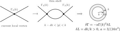
A shell of positive thickness $\delta L=\log[k/(k-dk)]$ corrects the local four-point vertex by $\delta\Gamma=-a\Gamma^2\delta L$. In the differential limit, $dL=-d\log k$, so $k\,d\Gamma/dk=a\Gamma^2$.

The same statement can be written as an integral equation. Starting at the bare cutoff,

$$\Gamma_4(\Lambda)=\lambda_0,$$

and integrating all shells between $q$ and $\Lambda$ gives

$$\boxed{ \Gamma_4(q)=\lambda_0-a\int_q^\Lambda {dk\over k}\,\Gamma_4(k)^2. }$$

This equation is the leading-log approximation in its most useful form. It says that the vertex at scale $q$ equals the bare vertex minus the sum of all logarithmic shell corrections above $q$. The coefficient contains the three four-point channels, the bubble symmetry factor $1/2$, and the radial shell factor $1/(8\pi^2)$. Because each shell needs only the subdivergence-subtracted local vertex at that shell, the equation is first order in the scale.

A quick consistency check recovers the one-loop result. Replace $\Gamma_4(k)$ under the integral by $\lambda_0$:

$$\Gamma_4(q)=\lambda_0-a\lambda_0^2\int_q^\Lambda {dk\over k}+\cdots =\lambda_0-a\lambda_0^2\log{\Lambda\over q}+\cdots.$$

The next iteration automatically produces the two-loop leading logarithm, and so on.

Solving the RG equation

Let

$$t=\log k.$$

The RG equation is

$${d\Gamma\over dt}=a\Gamma^2.$$

It is easier to solve after inverting the coupling:

$${d\over dt}\left({1\over\Gamma}\right) =-{1\over\Gamma^2}{d\Gamma\over dt} =-a.$$

Therefore

$${1\over\Gamma(k)}={1\over\Gamma(\Lambda)}+a\log{\Lambda\over k}.$$

Using $\Gamma(\Lambda)=\lambda_0$, we find

$$\boxed{ {1\over\Gamma_4(q)}={1\over\lambda_0}+a\log{\Lambda\over q} }$$

or

$$\boxed{ \Gamma_4(q)={\lambda_0\over1+a\lambda_0\log(\Lambda/q)}. }$$

Expanding the denominator gives

$$\Gamma_4(q) =\lambda_0\left[1-a\lambda_0 L+a^2\lambda_0^2L^2-a^3\lambda_0^3L^3+\cdots\right], \qquad L=\log{\Lambda\over q}.$$

Thus

$$\Gamma_4(q)=\lambda_0-a\lambda_0^2L+a^2\lambda_0^3L^2-a^3\lambda_0^4L^3+\cdots.$$

This is exactly the leading-log series anticipated from nested subgraphs. The differential equation is a compact way to sum the logarithmic simplex volumes and the vertex-renormalization factors at all orders.

What the sign means

For positive $\lambda_0$, the denominator

$$1+a\lambda_0\log{\Lambda\over q}$$

increases as $q$ is lowered. Hence

$$q\ll\Lambda \quad\Longrightarrow\quad \Gamma_4(q)<\lambda_0.$$

On the critical trajectory, the repulsive scalar interaction becomes weaker in the infrared. The four-dimensional $\phi^4$ coupling is marginally irrelevant at the Gaussian fixed point: it is marginal by engineering dimension, but quantum fluctuations make it drift logarithmically toward zero at long distances. A fixed massive theory instead leaves this scaling regime. In the massive fixed-input four-point example, the one-loop external-momentum derivative is suppressed at low momentum and the vertex approaches a finite, generally nonzero constant. That example fixes the Euclidean MOM mass by $\Gamma^{(2)}(0)=m_{\rm MOM}^2$; it is not a general definition of an exact pole mass or inverse exponential correlation length. At the retained one-loop order with the stated field normalization, these mass definitions agree; beyond it they must be distinguished.

The same equation says that the coupling grows as we move toward the ultraviolet. If we define a coupling $\lambda_R$ at a reference scale $\mu$, then

$${1\over\Gamma_4(q)}={1\over\lambda_R}+a\log{\mu\over q}, \qquad \lambda_R\equiv\Gamma_4(\mu).$$

For $q>\mu$, this is

$$\Gamma_4(q)={\lambda_R\over1-a\lambda_R\log(q/\mu)}.$$

The denominator vanishes at

$$q=\mu_{\mathrm{LP}} =\mu\exp\left({1\over a\lambda_R}\right).$$

This is the perturbative Landau pole. It does not mean that the one-loop approximation can be trusted all the way to the pole; the coupling becomes large before the pole is reached. It does mean that perturbation theory itself gives no evidence for an interacting ultraviolet-complete four-dimensional scalar theory with positive coupling.

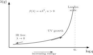
Schematic leading-log running for $a>0$ and positive $\lambda$ on the massless critical trajectory. The coupling decreases toward the infrared; this is not the low-momentum curve of a fixed massive theory. The formal ultraviolet solution has a Landau pole, but perturbation theory fails before that scale is reached.

A negative scalar coupling would formally run toward zero in the ultraviolet, but the Euclidean potential would be unbounded below. That is not the same kind of asymptotic freedom as non-Abelian Yang–Mills theory, where the stable positive gauge coupling has a negative beta function for $g$ at small $g$.

The same sign information can be summarized as

$$\begin{array}{c|c|c} \text{scale variable} & \text{equation} & \text{positive }\lambda\text{ does what?} \\ \hline q\text{ increasing} & q\,d\lambda/dq=+a\lambda^2 & \text{grows toward the UV} \\ L=\log(\Lambda/q)\text{ increasing} & d\lambda/dL=-a\lambda^2 & \text{decreases toward the IR} \\ \mu\text{ increasing at fixed bare data} & \beta(\lambda)=+a\lambda^2 & \text{grows with the subtraction scale} \end{array}$$

Most sign mistakes in this calculation come from switching between $q$ and $L$ without changing the derivative.

Changing the cutoff

The cutoff $\Lambda$ is not a physical observable. It is a resolution scale used to separate explicitly retained modes from unresolved modes. If we lower the cutoff from $\Lambda$ to $\Lambda'$, with

$$q<\Lambda'<\Lambda,$$

we should be able to choose a new bare coupling $\lambda_0'$ at the lower cutoff so that the same low-energy vertex is obtained.

The running solution gives

$$\Gamma_4(q;\lambda_0,\Lambda) ={1\over {1/\lambda_0}+a\log(\Lambda/q)}.$$

Define the new bare coupling at $\Lambda'$ by matching the old theory at that scale:

$$\lambda_0'\equiv \Gamma_4(\Lambda';\lambda_0,\Lambda).$$

Then

$${1\over\lambda_0'}={1\over\lambda_0}+a\log{\Lambda\over\Lambda'}.$$

Now run from $\Lambda'$ down to $q$:

$$\Gamma_4(q;\lambda_0',\Lambda') ={1\over {1/\lambda_0'}+a\log(\Lambda'/q)}.$$

Substituting the expression for $1/\lambda_0'$ gives

$$\Gamma_4(q;\lambda_0',\Lambda') ={1\over {1/\lambda_0}+a\log(\Lambda/\Lambda')+a\log(\Lambda'/q)} ={1\over {1/\lambda_0}+a\log(\Lambda/q)}.$$

Thus

$$\boxed{ \Gamma_4(q;\lambda_0',\Lambda')=\Gamma_4(q;\lambda_0,\Lambda). }$$

This is the composition law of the retained leading-log flow. Running from $\Lambda$ to $q$ is equivalent to running through $\Lambda'$ with the coupling updated there. The algebra is exact for this one-coupling approximation; it does not equate complete blocked actions after changing only one parameter. A leading local description requires external momenta well below the new matching cutoff.

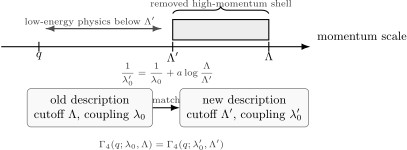
At leading-log accuracy, changing the cutoff from $\Lambda$ to $\Lambda'$ is compensated by changing the coupling from $\lambda_0$ to $\lambda_0'$. For probes with $q\ll\Lambda'$, the retained leading local contribution of the removed shell is absorbed into that coupling; higher-derivative terms and finite matching corrections are outside this approximation.

The word “group” in renormalization group is historically a little generous: with irreversible coarse graining, one naturally obtains a semigroup because integrating out modes cannot generally be inverted. In perturbative continuum calculations, however, the flow equations can often be run formally in either direction as long as the coupling remains small.

This also explains why a cutoff is not the same thing as a renormalization scale. A cutoff says which modes are explicitly present in a Wilsonian action. A renormalization scale $\mu$ is a reference point at which a coupling is defined by a condition. In perturbation theory they are often moved together for convenience, but conceptually they answer different questions.

Renormalized coupling and the beta function

Instead of using the bare coupling at $\Lambda$, choose a renormalized coupling at a finite reference scale $\mu$:

$$\lambda_R\equiv\Gamma_4(\mu).$$

From the solution,

$${1\over\lambda_R}={1\over\lambda_0}+a\log{\Lambda\over\mu}.$$

Subtracting this from the equation for $\Gamma_4(q)$ gives

$$\boxed{ {1\over\Gamma_4(q)}={1\over\lambda_R}+a\log{\mu\over q}. }$$

Equivalently,

$$\boxed{ \Gamma_4(q)={\lambda_R\over1+a\lambda_R\log(\mu/q)}. }$$

Within the critical or above-mass window, choosing $\mu\sim q$ avoids a large logarithm in the fixed-order boundary calculation. Choosing another $\mu$ reproduces the same leading logarithms by running $\lambda_R$. This scale choice does not supply omitted finite matching terms or extend the massless momentum formula below a nonzero mass scale.

The beta function is the derivative of the renormalized coupling with respect to the reference scale at fixed bare parameters:

$$\beta(\lambda_R) =\mu{\partial\lambda_R\over\partial\mu}\bigg|_{\lambda_0,\Lambda}.$$

Using

$$\lambda_R={\lambda_0\over1+a\lambda_0\log(\Lambda/\mu)},$$

we get

$$\boxed{ \beta(\lambda_R)=a\lambda_R^2+O(\lambda_R^3). }$$

In this massless leading-log approximation, the equation has the same form with $q$ replaced by the reference scale $\mu$. A mass-independent subtraction-scale coupling can continue running below a mass threshold without describing the massive vertex’s momentum dependence there. The Callan–Symanzik mass-insertion term explains why momentum dilation and fixed-bare subtraction-scale evolution differ when a mass is present.

This is also visible from counterterms. To first nontrivial order,

$$\lambda_R=\lambda_0-a\lambda_0^2\log{\Lambda\over\mu}+O(\lambda_0^3),$$

so the inverse relation is

$$\lambda_0=\lambda_R+a\lambda_R^2\log{\Lambda\over\mu}+O(\lambda_R^3).$$

Holding $\lambda_0$ fixed and differentiating with respect to $\log\mu$ gives, through order $\lambda_R^2$,

$$0=\beta(\lambda_R)-a\lambda_R^2+O(\lambda_R^3),$$

hence

$$\beta(\lambda_R)=a\lambda_R^2+O(\lambda_R^3).$$

The cutoff logarithm and the beta function are two ways of reading the same short-distance coefficient.

Scheme dependence and what is universal here

The coefficient

$$a={3\over16\pi^2}$$

is tied to the normalization $S_E\supset\int d^4x\,\lambda\phi^4/4!$. Rescaling the coupling changes this coefficient. With the leading normalization fixed, it is invariant under scale-independent analytic finite redefinitions in the massless or mass-independent setting considered here. This does not assert an unchanged external-momentum derivative across a massive threshold.

For example, suppose two definitions of the coupling differ by a finite redefinition with scale-independent constant $c$:

$$\lambda'=\lambda+c\lambda^2+O(\lambda^3).$$

Then

$$\beta'(\lambda')={d\lambda'\over d\lambda}\beta(\lambda) =(1+2c\lambda+\cdots)(a\lambda^2+b\lambda^3+\cdots).$$

Re-expressing the result in terms of $\lambda'$ gives

$$\beta'(\lambda')=a\lambda'^2+O(\lambda'^3).$$

The displayed one-loop coefficient is unchanged. If the finite redefinition instead depends explicitly on a mass-to-scale ratio, its scale derivative contributes and the chain rule must include that term. No higher-order universality claim follows without specifying the class of schemes and redefinitions.

At leading-log order, the distinction is simple. Finite constants in a one-loop amplitude change terms of order $\lambda^2$ with no large logarithm. They are not part of the leading-log series

$$\lambda(\lambda L)^n.$$

They become important when one goes to next-to-leading-log accuracy or wants a numerically precise prediction at a specified subtraction scheme.

Fixed point language

The RG equation

$${d\Gamma\over d\log\mu}=a\Gamma^2$$

has a fixed point at

$$\Gamma_*=0.$$

Linearization is inconclusive because

$$\beta'(0)=0.$$

The quadratic term decides the fate of this engineering-marginal coupling. For $a>0$ and $\Gamma>0$, increasing $\mu$ increases it, while decreasing $\mu$ decreases it. On the tuned critical trajectory, the Gaussian fixed point is attractive in the infrared along the positive $\phi^4$ direction and repulsive in the ultraviolet. A nonzero relevant mass sends the physical long-distance theory away from that trajectory.

The flow is logarithmically slow. For $\mu<\mu_0$,

$$\Gamma(\mu)={\Gamma(\mu_0)\over1+a\Gamma(\mu_0)\log(\mu_0/\mu)}.$$

Along the critical trajectory, at very low scales,

$$\Gamma(\mu)\sim {1\over a\log(\mu_0/\mu)}.$$

This slow decay is the source of logarithmic corrections to scaling near four-dimensional critical points. The next page uses this same running-coupling logic in thermodynamic quantities.

Generalization to O(N)

The scalar theory often appears with $N$ real fields and $O(N)$ symmetry:

$$S_E=\int d^4x\left[{1\over2}(\partial_\mu\phi_i)^2+{1\over2}m^2\phi_i^2+{\lambda\over4!}(\phi_i\phi_i)^2\right].$$

The same critical mass tuning and leading-log regime are assumed; again, the cutoff coefficient $m^2$ need not itself be zero. Hard subgraphs contribute their leading local terms, and a first-order RG equation sums the leading logarithms. Only the combinatorial coefficient changes. With the normalization above, the one-loop beta function is

$$\beta(\lambda)={N+8\over48\pi^2}\lambda^2+O(\lambda^3).$$

For $N=1$ this reduces to

$${9\over48\pi^2}={3\over16\pi^2},$$

as used throughout this page. The $N+8$ factor counts the internal index contractions in the three four-point channels. Later, the $O(N)$ model will reappear in a much more powerful form through large-$N$ methods and nonlinear sigma models.

A first operator insertion: φ²

The same shell logic also applies to local operator insertions. The simplest example is the quadratic operator

$$O(x)={1\over2}\phi(x)^2.$$

Linearize in a source for this operator about the critical background. A constant source is a mass perturbation:

$$\delta S_E=\int d^4x\,r_0 O(x).$$

The source $r_0$ has a power-law scaling because $O$ is relevant, with logarithmic corrections from the marginal $\phi^4$ interaction. To isolate those corrections, define $\tau(q)$ as the dimensionless leading local insertion factor at a positive Wilsonian/RG scale $q$, normalized by

$$\tau(\Lambda)=1.$$

At leading-log order, one $\phi^4$ vertex renormalizes this local factor through shells between the positive lower scale $q$ and $\Lambda$. That lower scale is the infrared prescription. A constant source transfers zero momentum: nonzero scalar-leg momenta alone would not regulate the full massless zero-transfer insertion bubble. We compute the local shell factor, not that full vertex. Each shell uses $\Gamma_4(k)$ and $\tau(k)$, giving

$$\tau(q)=1-b\int_q^\Lambda {dk\over k}\,\Gamma_4(k)\tau(k), \qquad b={1\over16\pi^2}.$$

Here $b$ denotes the one-loop insertion coefficient, distinct from the generic higher-order coefficient in the scheme example. The sign follows the same effective-action convention as the four-point vertex. Differentiating gives

$$q{d\tau(q)\over dq}=b\,\Gamma_4(q)\tau(q).$$

Equivalently, with $L=\log(\Lambda/q)$,

$${d\tau\over dL}=-b\,\Gamma_4(L)\tau.$$

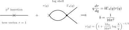
A $\phi^2$ insertion has two external scalar legs. A logarithmic shell with one $\phi^4$ vertex renormalizes the insertion by an amount proportional to $\Gamma_4(k)\tau(k)$.

Using

$$\Gamma_4(L)={\lambda_0\over1+a\lambda_0L}, \qquad a={3\over16\pi^2},$$

we find

$${d\log\tau\over dL} =-{b\lambda_0\over1+a\lambda_0L}.$$

Thus

$$\log\tau(L)=-{b\over a}\log(1+a\lambda_0L),$$

and therefore

$$\boxed{ \tau(q)=\left(1+{3\lambda_0\over16\pi^2}\log{\Lambda\over q}\right)^{-1/3}. }$$

The exponent $1/3$ is the ratio

$${b\over a}={1/(16\pi^2)\over3/(16\pi^2)}={1\over3}.$$

This is the first glimpse of anomalous dimensions in these notes. The coefficient multiplying a local operator, and the normalization assigned to the operator itself, run with scale. Which factor is called “source renormalization” and which factor is called “operator renormalization” is a convention; their product in correlation functions is physical.

What has been ignored

The four-point vertex is the cleanest place to see the RG because, in four-dimensional $\phi^4$ theory, the coupling is marginal and logarithmic already at one loop. Several complications have deliberately been postponed.

First, the relevant mass has been tuned for the critical calculation; coupling evolution does not perform that tuning. Away from the critical trajectory, the physical mass limits the scaling window. Mass tuning and its stopping scale distinguishes the cutoff parameter, critical shift and physical correlation length.

Second, wavefunction renormalization in $\phi^4$ theory starts later than the four-point coupling. At one loop the self-energy is momentum independent, so the leading one-loop logarithm for the four-point vertex is not accompanied by a one-loop anomalous dimension for $\phi$.

Third, the full four-point amplitude has channel dependence. The local coupling $\Gamma_4(q)$ is a convenient projection onto the marginal local operator. Nonlocal logarithms in particular kinematic channels matter for scattering amplitudes, but the RG equation for the local coupling is extracted by a specified subtraction prescription.

Fourth, a massive external-momentum vertex has threshold dependence even in Euclidean kinematics, while exceptional massless configurations can have additional infrared singularities. The positive-scale shell factors here isolate leading logarithms; they do not compute every finite or nonlocal part of those vertices.

These caveats are not defects. They are the reason the Wilsonian viewpoint is useful: it tells us which parts of a calculation are universal local running, which parts are matching, and which parts belong to other operators.

Summary

The one-loop logarithm in four-dimensional $\phi^4$ theory has coefficient

$$a={3\over16\pi^2}$$

in the normalization $S_E\supset\int d^4x\,\lambda\phi^4/4!$.

On the critical trajectory, or within the massive theory’s above-mass scaling window, an infinitesimal shell contributes the leading local correction proportional to $\Gamma_4(k)^2d\log k$. At leading-log accuracy this gives

$${d\Gamma_4\over d\log k}=a\Gamma_4^2, \qquad \Gamma_4(\Lambda)=\lambda_0.$$

Solving the equation gives

$$\Gamma_4(q)={\lambda_0\over1+a\lambda_0\log(\Lambda/q)}.$$

Expanding this result reproduces the leading-log tower

$$\lambda_0-a\lambda_0^2L+a^2\lambda_0^3L^2-\cdots.$$

Changing the cutoff is compensated by changing the bare coupling according to

$${1\over\lambda_0'}={1\over\lambda_0}+a\log{\Lambda\over\Lambda'}.$$

The low-energy vertex is unchanged because RG flow has a composition law.

If $\lambda_R=\Gamma_4(\mu)$, the beta function is

$$\beta(\lambda_R)=\mu{\partial\lambda_R\over\partial\mu}=a\lambda_R^2+O(\lambda_R^3).$$

Positive $\phi^4$ coupling is marginally irrelevant along the massless critical trajectory and grows toward the ultraviolet. The formal Landau pole lies beyond perturbative control. A fixed massive momentum-space vertex instead approaches a finite low-momentum value; continuing a mass-independent subtraction scale below its mass is a different operation.

The same shell idea renormalizes the local $\phi^2$ insertion factor at positive scale, linearized about the critical background. With $O=\phi^2/2$, it obeys

$$q{d\tau\over dq}={1\over16\pi^2}\Gamma_4(q)\tau,$$

so

$$\tau(q)=\left(1+{3\lambda_0\over16\pi^2}\log{\Lambda\over q}\right)^{-1/3}.$$

Common pitfalls

Changing the flow variable changes the displayed sign. Within the stated critical leading-log momentum interpretation and matching condition $\Gamma_4(\Lambda)=\lambda_0$, the equation is

$$q{\partial\Gamma_4\over\partial q}=a\Gamma_4^2,$$

while lowering $q$ makes $\Gamma_4$ smaller for positive coupling.

Bare and renormalized couplings are different data. The bare coupling $\lambda_0$ depends on the cutoff when a specified renormalized input $\lambda_R$ is held fixed. A subtraction-scale derivative is not automatically the external-momentum derivative of a massive vertex.

The Landau pole is not a controlled strong-coupling prediction. It is a perturbative obstruction, and the one-loop approximation fails before the pole is reached.

Do not add nested subgraphs twice. Their local effects are already contained in $\Gamma_4(k)$. The leading two-loop logarithm is generated by iterating the one-loop shell correction, while primitive two-loop graphs enter at lower logarithmic accuracy.

Coupling normalization fixes the numerical coefficient. The value $3/(16\pi^2)$ assumes the interaction is $\lambda\phi^4/4!$ for one real scalar field.

Source and operator factors are inverse conventions. If a source multiplying $O$ runs with one factor, the conventionally normalized operator carries the inverse factor so that their product is unchanged.

Exercises

Exercise 1 — Solving and expanding the flow

Solve

$${d\Gamma\over d\log q}=a\Gamma^2, \qquad \Gamma(\Lambda)=\lambda_0,$$

and expand the answer through order $\lambda_0^4$.

Solution

Invert the coupling:

$${d\over d\log q}\left({1\over\Gamma}\right) =-a.$$

Integrating from $\Lambda$ to $q$ gives

$${1\over\Gamma(q)}-{1\over\Gamma(\Lambda)} =-a\log{q\over\Lambda} =a\log{\Lambda\over q}.$$

Since $\Gamma(\Lambda)=\lambda_0$,

$${1\over\Gamma(q)}={1\over\lambda_0}+a\log{\Lambda\over q}.$$

Thus

$$\Gamma(q)={\lambda_0\over1+a\lambda_0L}, \qquad L=\log{\Lambda\over q}.$$

Expanding,

$$\Gamma(q)=\lambda_0\left(1-a\lambda_0L+a^2\lambda_0^2L^2-a^3\lambda_0^3L^3+\cdots\right).$$

Therefore through order $\lambda_0^4$,

$$\Gamma(q)=\lambda_0-a\lambda_0^2L+a^2\lambda_0^3L^2-a^3\lambda_0^4L^3+O(\lambda_0^5L^4).$$

Exercise 2 — Sliding-cutoff invariance

Let

$$\Gamma(q;\lambda_0,\Lambda) ={1\over {1/\lambda_0}+a\log(\Lambda/q)}.$$

Choose $\Lambda'$ with $q<\Lambda'<\Lambda$ and define

$$\lambda_0'=\Gamma(\Lambda';\lambda_0,\Lambda).$$

Show that

$$\Gamma(q;\lambda_0',\Lambda')=\Gamma(q;\lambda_0,\Lambda).$$

Solution

By definition,

$$\lambda_0'={1\over {1/\lambda_0}+a\log(\Lambda/\Lambda')}.$$

Thus

$${1\over\lambda_0'}={1\over\lambda_0}+a\log{\Lambda\over\Lambda'}.$$

Running from $\Lambda'$ to $q$ gives

$$\Gamma(q;\lambda_0',\Lambda') ={1\over {1/\lambda_0'}+a\log(\Lambda'/q)}.$$

Substitute $1/\lambda_0'$:

$$\Gamma(q;\lambda_0',\Lambda') ={1\over {1/\lambda_0}+a\log(\Lambda/\Lambda')+a\log(\Lambda'/q)}.$$

Since

$$\log{\Lambda\over\Lambda'}+\log{\Lambda'\over q}=\log{\Lambda\over q},$$

we obtain

$$\Gamma(q;\lambda_0',\Lambda') ={1\over {1/\lambda_0}+a\log(\Lambda/q)} =\Gamma(q;\lambda_0,\Lambda).$$

Exercise 3 — Beta function from the bare coupling

Suppose the bare and renormalized couplings are related at one loop by

$$\lambda_0=\lambda_R+a\lambda_R^2\log{\Lambda\over\mu}+O(\lambda_R^3).$$

Holding $\lambda_0$ and $\Lambda$ fixed, derive

$$\beta(\lambda_R)=\mu{\partial\lambda_R\over\partial\mu}=a\lambda_R^2+O(\lambda_R^3).$$

Solution

Differentiate the relation with respect to $\log\mu$ at fixed $\lambda_0$ and $\Lambda$:

$$0={d\lambda_R\over d\log\mu} +a{d\over d\log\mu}\left(\lambda_R^2\log{\Lambda\over\mu}\right) +O(\lambda_R^3).$$

Let

$$\beta(\lambda_R)={d\lambda_R\over d\log\mu}.$$

Then

$${d\over d\log\mu}\left(\lambda_R^2\log{\Lambda\over\mu}\right) =2\lambda_R\beta(\lambda_R)\log{\Lambda\over\mu}-\lambda_R^2.$$

The first term is of order $\lambda_R\beta$. Since $\beta$ begins at order $\lambda_R^2$, this term is $O(\lambda_R^3)$ and can be dropped at one-loop order. Therefore

$$0=\beta(\lambda_R)-a\lambda_R^2+O(\lambda_R^3),$$

so

$$\beta(\lambda_R)=a\lambda_R^2+O(\lambda_R^3).$$

Exercise 4 — The scalar Landau pole and infrared flow

Use the massless critical leading-log flow with $a=3/(16\pi^2)$ and a weak positive input $\lambda_R$ at scale $\mu$. Find the formal perturbative Landau-pole scale $\mu_{\rm LP}$. After the infinite-volume limit, approach $q\to0$ through nonzero nonexceptional Euclidean four-point configurations with fixed channel ratios. What happens to the coupling along this tuned trajectory, rather than at fixed positive mass?

Solution

For $q>\mu$,

$$\Gamma(q)={\lambda_R\over1-a\lambda_R\log(q/\mu)}.$$

The denominator vanishes when

$$1-a\lambda_R\log{q\over\mu}=0.$$

Thus

$$\mu_{\rm LP}=\mu\exp\left({1\over a\lambda_R}\right).$$

For $q<\mu$,

$$\Gamma(q)={\lambda_R\over1+a\lambda_R\log(\mu/q)}.$$

As $q\to0$, the logarithm grows and

$$\Gamma(q)\sim {1\over a\log(\mu/q)}\to0.$$

The coupling is marginally irrelevant in the infrared.

Exercise 5 — Universality under a finite redefinition

A finite redefinition with scale-independent constant $c$ is given by

$$\lambda'=\lambda+c\lambda^2+O(\lambda^3).$$

If

$$\beta(\lambda)=a\lambda^2+b\lambda^3+O(\lambda^4),$$

show that the coefficient of $\lambda'^2$ in $\beta'(\lambda')$ is still $a$.

Solution

By the chain rule,

$$\beta'(\lambda')={d\lambda'\over d\lambda}\beta(\lambda).$$

Since

$${d\lambda'\over d\lambda}=1+2c\lambda+O(\lambda^2),$$

we have

$$\beta'(\lambda')=(1+2c\lambda+\cdots)(a\lambda^2+b\lambda^3+\cdots) =a\lambda^2+O(\lambda^3).$$

To find the coefficient of the quadratic term in $\lambda'$, we only need

$$\lambda=\lambda'+O(\lambda'^2).$$

Therefore

$$\beta'(\lambda')=a\lambda'^2+O(\lambda'^3).$$

The one-loop coefficient is unchanged by a finite redefinition of the coupling.

Exercise 6 — The O(N) one-loop flow

For the $O(N)$ theory

$$S_E\supset\int d^4x\,{\lambda\over4!}(\phi_i\phi_i)^2,$$

the one-loop beta function is

$$\beta(\lambda)={N+8\over48\pi^2}\lambda^2+O(\lambda^3).$$

Check that this formula reproduces the coefficient used on this page for $N=1$. Then write the leading-log solution for general $N$.

Solution

For $N=1$,

$${N+8\over48\pi^2}={9\over48\pi^2}={3\over16\pi^2},$$

which is the coefficient

$$a={3\over16\pi^2}$$

used for a single real scalar.

For general $N$, define

$$a_N={N+8\over48\pi^2}.$$

The leading-log RG equation is

$${d\lambda\over d\log q}=a_N\lambda^2, \qquad \lambda(\Lambda)=\lambda_0.$$

Solving as before gives

$$\lambda(q)={\lambda_0\over1+a_N\lambda_0\log(\Lambda/q)}.$$

Exercise 7 — Running of the quadratic insertion

Let $\tau(q)$ satisfy

$$q{d\tau\over dq}=b\Gamma(q)\tau, \qquad \tau(\Lambda)=1,$$

where

$$\Gamma(q)={\lambda_0\over1+a\lambda_0\log(\Lambda/q)}.$$

Show that

$$\tau(q)=\left(1+a\lambda_0\log{\Lambda\over q}\right)^{-b/a}.$$

Then evaluate the exponent for $a=3/(16\pi^2)$ and $b=1/(16\pi^2)$.

Solution

Set

$$L=\log{\Lambda\over q}.$$

Then

$$q{d\over dq}=-{d\over dL},$$

so the differential equation becomes

$${d\tau\over dL}=-b\,{\lambda_0\over1+a\lambda_0L}\tau.$$

Divide by $\tau$:

$${d\log\tau\over dL}=-{b\lambda_0\over1+a\lambda_0L}.$$

Integrating from $0$ to $L$ and using $\tau(0)=1$ gives

$$\log\tau(L)=-b\int_0^L {\lambda_0\,dL'\over1+a\lambda_0L'}.$$

The integral is

$$\int_0^L {\lambda_0\,dL'\over1+a\lambda_0L'}={1\over a}\log(1+a\lambda_0L),$$

so

$$\tau(L)=\left(1+a\lambda_0L\right)^{-b/a}.$$

For

$$a={3\over16\pi^2}, \qquad b={1\over16\pi^2},$$

we have

$${b\over a}={1\over3},$$

and hence

$$\tau(q)=\left(1+{3\lambda_0\over16\pi^2}\log{\Lambda\over q}\right)^{-1/3}.$$

Further reading

• Coleman, Sidney. Lectures of Sidney Coleman on Quantum Field Theory. Edited by Bryan Gin-ge Chen, David Derbes, David Griffiths, Brian Hill, Richard Sohn, and Yuan-Sen Ting. World Scientific, 2019.
• Schwartz, Matthew D. Quantum Field Theory and the Standard Model. Cambridge University Press, 2014.
• Srednicki, Mark. Quantum Field Theory. Cambridge University Press, 2007.
• Weinberg, Steven. The Quantum Theory of Fields, Volume II: Modern Applications. Cambridge University Press, 1996.
• Zinn-Justin, Jean. Quantum Field Theory and Critical Phenomena. 4th ed. Oxford University Press, 2002.