Two-Dimensional QED, the Thirring Model, and Currents

A current Ward identity fixes how a symmetry acts on operator insertions. In two dimensions it also gives a particularly direct route to dynamics: for one massless Dirac fermion, the vector-preserving axial anomaly and Maxwell equation imply the electric-field mass $m_\gamma^2=e^2/\pi$. A local Thirring interaction has a different effect: in its massless, positive-stiffness regime it changes scaling dimensions along a line of conformal theories.

This lesson develops both calculations with the same chiral-current normalization. The background-source and current-algebra arguments are Euclidean; the physical anomaly and electric-field equation are Lorentzian. The Schwinger calculation concerns the massless theory on the line, with boundary and zero-mode qualifications stated below. It does not describe the massive Schwinger model or every finite-volume gauge sector.

Required background. Lesson 19 supplies current Ward identities, contact terms and the distinction between a transverse self-energy and a local mass tensor. Helpful background. Lesson 10 develops two-dimensional chiral equations; Lesson 17 explains the continuation and normalization of a chiral fermion.

Chiral amplitudes and current normalization

Use the global 1+1-dimensional Clifford, orientation and light-cone conventions. To display the spinor components explicitly, choose $\gamma^0=\sigma_1$ and $\gamma^1=-i\sigma_2$, so $\gamma_*=\sigma_3$. Write the Dirac field in terms of one-component Grassmann amplitudes:

$$\Psi= \begin{pmatrix}\chi_-\\ \chi_+\end{pmatrix}, \qquad P_+\Psi=\begin{pmatrix}\chi_-\\0\end{pmatrix}, \qquad P_-\Psi=\begin{pmatrix}0\\\chi_+\end{pmatrix}.$$

The subscripts on $\chi_\pm$ label propagation coordinates, not projector eigenvalues. The amplitudes are numbers in spinor-component space; $P_\pm\Psi$ are two-component embedded spinors. This distinction matters for the mass bilinear later.

With the Cartesian measure $d^2x=dx^0dx^1$, the free Lorentzian action is

$$S_{0,L}=\int d^2x\, \left(2i\chi_+^\dagger\partial_-\chi_+ +2i\chi_-^\dagger\partial_+\chi_-\right).$$

The global derivatives and one-form components each contain a factor $1/2$. The equations and the associated number densities are

Amplitude	Embedded spinor	Free equation	Number density
$\chi_+$	$P_-\Psi$	$\partial_-\chi_+=0$; depends on $x^+$	$J_+=:\!\chi_+^\dagger\chi_+\!:$
$\chi_-$	$P_+\Psi$	$\partial_+\chi_-=0$; depends on $x^-$	$J_-=:\!\chi_-^\dagger\chi_-\!:$

Define $J_V^\mu=\bar\Psi\gamma^\mu\Psi$ and $J_A^\mu=\bar\Psi\gamma^\mu\gamma_*\Psi$. The global Clifford identity gives $J_A^\mu=-\epsilon^{\mu\nu}J_{V,\nu}$, or explicitly

$$\begin{aligned} J_V^0&=J_++J_-, &\qquad J_V^1&=-J_++J_-,\\ J_A^0&=-J_++J_-, & J_A^1&=J_++J_-. \end{aligned}$$

Consequently,

$$\begin{aligned} \partial_\mu J_V^\mu&=2(\partial_-J_++\partial_+J_-),\\ \partial_\mu J_A^\mu&=2(-\partial_-J_++\partial_+J_-),\\ A_\mu J_V^\mu&=2(A_-J_++A_+J_-). \end{aligned}$$

A vector rotation multiplies both amplitudes by $e^{i\alpha}$. An axial rotation multiplies $\chi_+$ by $e^{-i\beta_A}$ and $\chi_-$ by $e^{i\beta_A}$. In the free massless theory both currents are conserved, giving separate chiral conservation.

Complex Euclidean fermions

Let $x^0=-i\tau$, $z=x^1+i\tau$ and $d^2z=dx^1d\tau$. Then $\partial_+\to\bar\partial$ and $\partial_-\to-\partial$. Choose the constant field factors

$$\begin{aligned} \chi_-&\longrightarrow {e^{i\pi/4}\over\sqrt{2\pi}}\psi, &\quad \chi_-^\dagger&\longrightarrow {e^{i\pi/4}\over\sqrt{2\pi}}\psi^\dagger,\\ \chi_+&\longrightarrow {e^{-i\pi/4}\over\sqrt{2\pi}}\bar\psi, & \chi_+^\dagger&\longrightarrow {e^{-i\pi/4}\over\sqrt{2\pi}}\bar\psi^\dagger. \end{aligned}$$

The Euclidean dagger variables are independent Grassmann integration variables. Their continuation factors are therefore not obtained by complex-conjugating the factors on the undaggered fields. Likewise $\bar\psi$ names the other chiral field, not the complex conjugate of $\psi$.

Substitution in $e^{iS_L}=e^{-S_E}$ gives

$$S_{0,E}={1\over\pi}\int d^2z\, \left(\psi^\dagger\bar\partial\psi+ \bar\psi^\dagger\partial\bar\psi\right).$$

This coefficient is fixed by the required unit pole. For $K=\bar\partial/\pi$,

$$K_z\,{1\over z-w}=\delta^{(2)}(z-w), \qquad \bar\partial{1\over z-w}=\pi\delta^{(2)}(z-w),$$

so $\langle\psi(z)\psi^\dagger(w)\rangle=1/(z-w)$, and similarly in the antiholomorphic sector. A coefficient $1/(2\pi)$ multiplying this complex action would give twice that covariance. The real Majorana quadratic form in Lesson 17 has a different combinatorial factor. Combining two real fields as $\psi=(\rho_1+i\rho_2)/\sqrt2$ and $\psi^\dagger=(\rho_1-i\rho_2)/\sqrt2$, then integrating by parts with Grassmann signs, turns their two real actions into the complex action above. The real action and inverse kernel are given in Di Francesco et al. 1997, §5.3.2, pp.129–131, Eqs.5.88 and 5.93.

Define the residue-normalized Euclidean currents

$$J=:\!\psi^\dagger\psi\!:, \qquad \bar J=:\!\bar\psi^\dagger\bar\psi\!:.$$

Their relation to the physical Lorentzian densities follows from the same field factors:

$$J_-\longrightarrow {i\over2\pi}J, \qquad J_+\longrightarrow {-i\over2\pi}\bar J.$$

Background gauge fields and Ward contacts

For this lesson the rescaled connection has unit charge: $D_\mu=\partial_\mu-iA_\mu$, $\Psi\mapsto e^{i\alpha}\Psi$ and $A_\mu\mapsto A_\mu+\partial_\mu\alpha$. The parameter $e$ will appear in the Maxwell term. Thus this charge assignment differs from the electron convention $q_{\rm site}=-e$ used for the QED vertex in Lesson 19.

Continue the one-form itself, with $A_\tau^E=-iA_0^L$ and $A_x^E=A_1^L$. Its complex components obey

$$A_{\bar z}^E={A_x^E+iA_\tau^E\over2}=A_+^L, \qquad A_z^E={A_x^E-iA_\tau^E\over2}=-A_-^L.$$

The Euclidean source action is therefore

$$S_E[\psi,A]=S_{0,E} -{i\over\pi}\int d^2z\,(A_{\bar z}J+A_z\bar J).$$

This expression defines the source normalization; the OPE currents themselves have no extra $1/\pi$. In Cartesian components it is $S_{0,E}-i\int A_a j_E^a$, where

$$j_E^x={J+\bar J\over2\pi}, \qquad j_E^\tau={i(J-\bar J)\over2\pi}.$$

In particular the physical source response is not the bare functional derivative without its factor of $i$. For $W_E[A]=-\log Z[A]$ and this linear source coupling, $\delta W_E/\delta A_a=-i\langle j_E^a\rangle$.

Hold $A$ fixed and localize the vector phase rotation. The two chiral kinetic terms give

$$\delta S_E={i\over\pi}\int d^2z\, (J\bar\partial\alpha+\bar J\partial\alpha) =-{i\over\pi}\int d^2z\,\alpha(\bar\partial J+\partial\bar J).$$

For an insertion product $\mathcal O=\prod_i O_i(z_i)$ with $\delta_\alpha O_i=i q_{{\rm gauge},i}\alpha(z_i)O_i$, a regulator preserving vector symmetry gives $0=\langle\delta_\alpha\mathcal O\rangle-\langle\mathcal O\,\delta_\alpha S_E\rangle$. Thus, with local counterterms and composite contacts treated in the same prescription,

$$\left\langle(\bar\partial J+\partial\bar J)(z)\,\mathcal O\right\rangle =-\pi\sum_i q_{{\rm gauge},i}\, \delta^{(2)}(z-z_i)\langle\mathcal O\rangle.$$

Away from insertions this is conservation. In the free chiral sector it also fixes the residue of a contour surrounding an insertion. If $A$ is transformed together with the fermions, the source variation cancels the localized kinetic variation instead. That is background gauge covariance. Making $A$ dynamical introduces an additional equation of motion; it does not change the meaning of the charged-insertion contacts.

Dynamical gauge fields and the electric-field equation

Now integrate over $A_\mu$ as well as the fermions. In Lorentzian signature take

$$S_L=\int d^2x\, \left[\bar\Psi i\gamma^\mu(\partial_\mu-iA_\mu)\Psi -{1\over4e^2}F_{\mu\nu}F^{\mu\nu}\right], \qquad e>0.$$

Here $A_\mu=e A_\mu^{\rm can}$, where $A^{\rm can}$ has a canonically normalized Maxwell term; $e$ has mass dimension one. The interaction is $+A_\mu J_V^\mu$, so varying the connection gives

$${1\over e^2}\partial_\mu F^{\mu\nu}+J_V^\nu=0.$$

The left-hand side is an Euler–Lagrange operator, not an additional matter Noether current. In quantum correlation functions its insertions can have equation-of-motion contacts; gauge fixing and unphysical insertions also require their own terms. The physical equation used below applies in gauge-invariant correlators away from these contacts. Taking its divergence gives vector conservation because $F^{\mu\nu}$ is antisymmetric.

Treatment of the field	Operation	Result
Background connection	Localize a matter rotation with the source fixed	A current Ward identity, including charged-insertion contacts
Dynamical connection	Vary the integrated gauge field	A Maxwell equation relating the matter current to the field strength
Algebraic auxiliary field	Complete its quadratic form	A local four-fermion interaction, derived below

Axial anomaly and Schwinger mass

For one massless Dirac fermion, define the renormalized vector and axial currents in a prescription preserving vector gauge invariance. With the charge and orientation already fixed,

$$\partial_\mu J_V^\mu=0, \qquad \partial_\mu J_A^\mu=-{F_{01}\over\pi}.$$

These are quantum identities with their appropriate insertion contacts. Classically the second right-hand side vanishes. The anomaly can be computed as the regulated axial Jacobian, or equivalently as the unavoidable axial contact in the vector-preserving current two-point function. Its sign must be translated together with the charge convention.

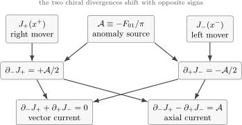
Write $E=F_{01}$ and $\mathcal A=-E/\pi$. The two chiral divergences obey

$$2(\partial_-J_++\partial_+J_-)=0, \qquad 2(-\partial_-J_++\partial_+J_-)=\mathcal A.$$

Therefore

$$\partial_-J_+=-{\mathcal A\over4}, \qquad \partial_+J_-={\mathcal A\over4}.$$

The factor $1/4$ follows from the global light-cone derivatives and the unrescaled physical number densities. A background electric field changes the two chiral charges oppositely while conserving vector charge.

For a dynamical field, the two Maxwell components give more information. Since $F^{10}=E$ and $F^{01}=-E$,

$$J_V^0=-{1\over e^2}\partial_1E, \qquad J_V^1={1\over e^2}\partial_0E.$$

The Clifford current identity then yields

$$J_A^0={1\over e^2}\partial_0E, \qquad J_A^1=-{1\over e^2}\partial_1E, \qquad J_A^\mu={1\over e^2}\partial^\mu E.$$

Combining its divergence with the anomaly gives

$${1\over e^2}\Box E=-{E\over\pi}, \qquad (\Box+m_\gamma^2)E=0, \qquad m_\gamma^2={e^2\over\pi}.$$

Thus the gauge-invariant electric-field excitation has $\omega^2=k^2+m_\gamma^2$ on the infinite line. The result uses both the anomaly and the dynamical Maxwell equation. The absence of a free Maxwell transverse photon polarization in $1+1$ dimensions does not exclude this matter-induced physical mode. A fermion mass would add an axial mass operator and invalidate this closed linear derivation.

The transverse kernel from a Gaussian scalar

The same mass appears in the nonzero-momentum effective action. Work on the Euclidean plane in the topologically trivial local sector. An infrared regulator can first restrict the calculation to a finite box with the scalar zero mode removed; the plane expression is understood on nonzero modes. Global gauge holonomies, topological sectors and boundary charges require separate treatment.

Bosonization represents the free massless Dirac vector current by a canonical Gaussian scalar $\varphi$:

$$S_{\varphi,E}={1\over2}\int d^2x\,(\partial_a\varphi)^2, \qquad j_E^a={1\over\sqrt\pi}\epsilon_E^{ab}\partial_b\varphi, \qquad \epsilon_E^{x\tau}=+1.$$

This is a current-sector representation, not an identification of a local fermion field with $\varphi$. It fixes the current two-point normalization, with the scalar’s sign chosen by the displayed map. The current/boson correspondence is specified in Coleman 1975, §I, pp.2088–2089, Eqs.1.4–1.10; the continuation and anomaly signs here follow from our charge and orientation. Its Lorentzian counterpart $J_V^\mu=-\epsilon^{\mu\nu}\partial_\nu\varphi/\sqrt\pi$ has $J_A^\mu=\partial^\mu\varphi/\sqrt\pi$; coupling it to $A$ gives $\Box\varphi=-E/\sqrt\pi$, reproducing the stated anomaly.

Set $F_E=F_{x\tau}$ and $Q=-\partial_E^2$. Integration by parts in the Euclidean linear source term gives

$$S_{\varphi,E}[A] ={1\over2}\int\varphi Q\varphi -{i\over\sqrt\pi}\int F_E\varphi.$$

Completing this convergent Gaussian at the regulated level and dividing by the zero-source integral gives

$$W_{\rm ferm}[A]-W_{\rm ferm}[0] ={1\over2\pi}\int F_E\,Q^{-1}F_E.$$

The positive sign follows from the imaginary Euclidean source: its square enters $\log Z$ with a minus sign. It is not a local Proca mass term. At $q_E^2>0$,

$$P^T_{ab}(q)=\delta_{ab}-{q_aq_b\over q_E^2}, \qquad W_{\rm ferm}[A]-W_{\rm ferm}[0] ={1\over2}\int {d^2q\over(2\pi)^2}\, A_a(-q){P^T_{ab}(q)\over\pi}A_b(q).$$

This quadratic response also agrees with the vector-preserving Pauli–Villars calculation in Morais and Mota 2009, arXiv v1, §II, p.2, and §V, p.8, Eqs.42–48, PDF. Their canonical gauge field has a factor $e^2$ in its polarization; rescaling to the unit connection removes it. The Gaussian-current argument above supplies the full local-sector source dependence, rather than inferring it from a two-point loop alone.

Adding the Maxwell action gives the transverse inverse kernel

$$\Gamma_{A,ab}^{T}(q)= \left({q_E^2\over e^2}+{1\over\pi}\right)P^T_{ab}(q).$$

After $A=eA^{\rm can}$, its eigenvalue is $q_E^2+m_\gamma^2$, consistent with the electric-field equation. The projector has no unique direction-independent value at the origin; the expression is not an inverse on the longitudinal gauge subspace. Gauge fixing supplies that separate subspace without altering the transverse pole.

The figure compares the transverse eigenvalues. Inspect their constant separation and the fact that both the anomaly and Maxwell equation enter the mass derivation.

For one massless Dirac fermion, the vector-preserving anomaly and dynamical Maxwell equation give $m_\gamma^2=e^2/\pi$. With $s=q_E^2/m_\gamma^2>0$ and $y=\pi\Gamma_{A,T}$, the plotted eigenvalues are $y=s$ and $y=s+1$. Open intercepts indicate eigenvalue limits, not a definition of the projector at zero momentum. The induced tensor is proportional to $P^T$, rather than the identity.

Local and nonlocal current interactions

The Thirring model uses a different quadratic field. Let $B_\pm$ be auxiliary variables, not components of a gauge connection, and let $g_L\ne0$. The algebraic action

$$S_{\rm aux}[B,J]=\int d^2x\, \left({B_+B_-\over g_L}-B_+J_--B_-J_+\right)$$

can be completed as

$$S_{\rm aux} =\int d^2x\, \left[{(B_+-g_LJ_+)(B_--g_LJ_-)\over g_L} -g_LJ_+J_-\right].$$

Stationary elimination, or the normalized Lorentzian Fresnel integral with a specified Gaussian prescription, therefore produces $-g_LJ_+J_-$. The indefinite real quadratic form is not an absolutely convergent Euclidean probability weight. A Euclidean auxiliary representation must choose its contour consistently. The free limit $g_L=0$ is defined directly in the fermion action.

The resulting Lorentzian theory is

$$\mathcal L_{\rm Th} =2i\chi_+^\dagger\partial_-\chi_+ +2i\chi_-^\dagger\partial_+\chi_- -g_LJ_+J_-.$$

Since $J_{V,\mu}J_V^\mu=4J_+J_-$ in the declared common composite prescription, the covariant notation is

$$\mathcal L_{\rm Th} =\bar\Psi i\gamma^\mu\partial_\mu\Psi -{g_T\over2}J_{V,\mu}J_V^\mu, \qquad g_L=2g_T.$$

This identity includes the normalization of the current product; it does not identify every regularization-dependent parameter called a Thirring coupling.

For comparison, eliminating a Euclidean Maxwell field uses an inverse differential operator. For a prescribed conserved source $j_E$ at $q_E^2>0$, its transverse kernel and inverse on that subspace are

$$K_A^T={q_E^2\over e^2}P^T, \qquad (K_A^T)^{-1}={e^2\over q_E^2}P^T.$$

The coupling $-i\int A_a j_E^a$ gives

$$S_{\rm induced}[j_E] ={e^2\over2}\int {d^2q\over(2\pi)^2}\, j_E^a(-q){P^T_{ab}(q)\over q_E^2}j_E^b(q).$$

The inversion is restricted to the conserved transverse sector, or performed after an actual gauge fixing. It is never an inverse of the singular Maxwell tensor on the full vector space. With the same infrared prescription, $Q^{-1}(x)=-\log(\mu|x|)/(2\pi)$ up to its arbitrary constant. This is the bare nonlocal current interaction. It does not imply an unscreened long-distance physical field after the fermions and gauge field are both integrated. The auxiliary Thirring kernel instead produces a local product.

Current algebra of a free chiral fermion

The holomorphic part of a free complex fermion has the short-distance OPE

$$\psi(z)\psi^\dagger(w)\sim {1\over z-w}.$$

Define the holomorphic $U(1)$ current

$$J(z)=:\!\psi^\dagger\psi\!:(z).$$

Contracting the dagger field through the intervening undaggered fermion supplies one minus sign, giving

$$J(z)\psi(w)\sim -{\psi(w)\over z-w}, \qquad J(z)\psi^\dagger(w)\sim +{\psi^\dagger(w)\over z-w}.$$

Thus $J$ measures the number charge: with $J=:\!\psi^\dagger\psi\!:$, annihilation and creation fields have charges $-1$ and $+1$, respectively. Reversing the overall sign of $J$ reverses all charges but leaves the physics unchanged. Double contraction gives the current-current OPE

$$\boxed{ J(z)J(w)\sim {1\over(z-w)^2}. }$$

More generally, an Abelian current algebra at level $k$ has

$$J(z)J(w)\sim {k\over(z-w)^2}.$$

The charge associated with a contour $C$ is

$$Q_C={1\over2\pi i}\oint_C dz\,J(z).$$

If $C$ surrounds an operator $O_{q_Q}(w)$ with contour-charge eigenvalue $q_Q$, then

$$J(z)O_{q_Q}(w)\sim {q_Q\over z-w}O_{q_Q}(w),$$

and therefore

$$Q_C O_{q_Q}(w)=q_QO_{q_Q}(w).$$

This contour formulation is the chiral version of the Ward identity. To connect it to the gauge phase fixed at the beginning of the page, we implement the transformation by

$$U(\alpha)=e^{-i\alpha Q}, \qquad \delta O=-i\alpha[Q,O].$$

Thus $[Q,\psi]=-\psi$ produces $\psi\mapsto e^{+i\alpha}\psi$: the contour eigenvalue is $q_Q=-1$, whereas the gauge-charge label in $D_\mu=\partial_\mu-iq_{\rm gauge}A_\mu$ is $q_{\rm gauge}=+1$. More generally, $q_Q=-q_{\rm gauge}$ with this implementation convention. Once this map is stated, a prescribed singular current OPE gives the Ward identities by contour deformation without a charge-sign ambiguity.

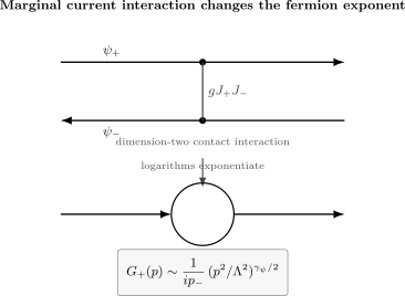
The Thirring model as a marginal deformation

The continuation factors above fix the coefficient of the normalized Euclidean current product:

$$S_{{\rm Th},E}=S_{0,E}+\kappa\int d^2z\,J\bar J, \qquad \kappa={g_L\over4\pi^2}={g_T\over2\pi^2}.$$

Here $J$ and $\bar J$ identify the currents of the undeformed free theory used to define the perturbation. The same letter $g_T$ cannot be assigned to this Euclidean coefficient without a conversion. The operator $J\bar J$ has free scaling dimension two; power counting therefore makes it marginal, but does not by itself prove exact marginality.

Gaussian stiffness and operator dimensions

Specify the vector-Ward-normalized current and current-product prescription used in Coleman’s equivalence. In this prescription the bosonized massless theory is

$$\mathcal L_{\varphi,L}={K\over2}(\partial_\mu\varphi)(\partial^\mu\varphi), \qquad K=1+{g_T\over\pi}=1+2\pi\kappa>0.$$

Indeed, the current representation $J_V^\mu=-\epsilon^{\mu\nu}\partial_\nu\varphi/\sqrt\pi$ gives $J_{V,\mu}J_V^\mu=-(\partial\varphi)^2/\pi$ in this composite prescription. Inserting it in the Thirring action changes the kinetic coefficient to $K$. This free Gaussian description establishes the exactly marginal massless line: changing a positive stiffness changes conformal dimensions without adding a scale. The fermion sector requires the corresponding bosonic vertex operators and zero-mode sectors, not merely a noncompact scalar polynomial algebra.

For the canonical scalar $\Phi=\sqrt K\,\varphi$, the renormalized mass vertex has coefficient

$$\beta^2={4\pi\over K}.$$

The statement includes the definition of the current: alternative Thirring current normalizations use a different coupling coordinate. Coleman’s normalization and equivalence are given in Coleman 1975, pp.2088–2089 and 2093, Eqs.1.4–1.9 and 4.22; his p.2097 note 7 explicitly distinguishes another current prescription.

The charged fermion is a vertex involving both $\Phi$ and its dual. Write $\Phi=\Phi_L+\Phi_R$ and $\widetilde\Phi=\Phi_L-\Phi_R$, with $\langle\Phi_L(z)\Phi_L(w)\rangle=-\log(z-w)/(4\pi)$. Up to its cocycle, normalization and choice of component, the fermion has vertex coefficients

$$a={\beta\over2}, \qquad b={2\pi\over\beta}, \qquad \psi\ \propto\ :\!\exp[-i(a\Phi+b\widetilde\Phi)]\!:.$$

The cocycle enforces the required anticommutation between distinct fermion components; it does not change the separated scaling dimension. Gaussian contraction gives

$$h={(a+b)^2\over8\pi}, \qquad \bar h={(a-b)^2\over8\pi},$$

and hence

$$\begin{aligned} \Delta_\psi&=h+\bar h ={\beta^2\over16\pi}+{\pi\over\beta^2} ={K+K^{-1}\over4},\\ s_\psi&=h-\bar h={1\over2}. \end{aligned}$$

The other component interchanges $h$ and $\bar h$. This operator construction and its conserved-current normalization are supported by Mandelstam 1975, pp.3027–3028, Eqs.2.8 and 3.6–3.10, translating his coupling by $g_M=-g_T$. The displayed Gaussian contractions explain the resulting dimensions rather than using the citation as a substitute for the calculation.

Only $K=1$ has $(h,\bar h)=(1/2,0)$ for this component. An interacting fermion is therefore not still a holomorphic free field with just a changed holomorphic weight. The currents can be represented by chiral Gaussian derivatives, while the charged fermion has both weights.

Correlation decay and anomalous dimension

Use the global field anomalous-dimension convention:

$$\gamma_{\rm site}=\Delta_\psi-\frac12 ={K+K^{-1}-2\over4} ={g_T^2\over4\pi^2K}\ge0.$$

Thus the first departure from the free fermion dimension is quadratic in $g_T$ in this prescription. For separated insertions,

$$\langle\psi(z,\bar z)\psi^\dagger(0)\rangle ={C\over z^{2h}\bar z^{2\bar h}}, \qquad z\ne0,$$

with a branch fixed consistently with the spin and radial ordering. Along a fixed ray, divide the magnitude by its value at $r_0>0$. The unknown amplitude and angular factor cancel:

$$R={r\over r_0}, \qquad C_\gamma(R)=R^{-1-2\gamma_{\rm site}}.$$

The figure shows how the exponent changes this measurable decay. Its three exponents illustrate the definition; they are not assigned to three particular coupling values.

Normalized two-point envelopes at illustrative $\gamma_{\rm site}=0,1/8,1/4$. The axes are $\ln R$ and $\ln C_\gamma$, so the slopes are $-1-2\gamma_{\rm site}$. The normalization at $r_0$ removes an unspecified component amplitude. These curves illustrate scaling; the coupling relation additionally requires the declared Thirring current prescription and $K>0$.

There is also a useful momentum check. For the component with spin $+1/2$, let $q_{\bar z}=(q_x+iq_\tau)/2$. At nonzero Euclidean momentum, in the range $0\le\gamma_{\rm site}<1/2$ where the separated position kernel is locally integrable, its Fourier transform has the form

$$G_\psi(q)\propto {1\over q_{\bar z}} \left({q_E^2\over\mu^2}\right)^{\gamma_{\rm site}}, \qquad G_\psi(\lambda q)=\lambda^{-1+2\gamma_{\rm site}}G_\psi(q), \quad \lambda>0.$$

An overall normalization and constant Fourier phase are suppressed. The positive Euclidean $q_E^2$ fixes the real power; a Lorentzian expression needs its separate continuation prescription. At larger dimensions the Fourier transform requires a distributional extension and local contact terms, so this simple representation is not assumed without qualification.

Expanding the nonlocal factor for small $\gamma_{\rm site}$ gives $1+\gamma_{\rm site}\log(q_E^2/\mu^2)+O(\gamma_{\rm site}^2)$. The exponent is $\gamma_{\rm site}$, not $\gamma_{\rm site}/2$.

Neutral mass operator and axial symmetry

The component distinction at the start now has a concrete use. Direct multiplication by $\gamma^0=\sigma_1$ gives

$$\bar\Psi\Psi=\chi_+^\dagger\chi_-+\chi_-^\dagger\chi_+.$$

These are nonzero products of one-component amplitudes. By contrast, $(P_-\Psi)^\dagger(P_+\Psi)=0$ by projector orthogonality; that expression is not the mass bilinear.

Each term is neutral under the vector rotation. Under the axial rotation, $\chi_+^\dagger\chi_-\mapsto e^{2i\beta_A}\chi_+^\dagger\chi_-$ and its conjugate has the opposite phase, where $\beta_A$ here denotes the axial angle. Thus a mass breaks the axial symmetry while preserving the vector symmetry. The free-field continuation gives the more precise normalization

$$-m\bar\Psi\Psi\ \hbox{in }\mathcal L_L \quad\longrightarrow\quad {m\over2\pi} (\bar\psi^\dagger\psi+\psi^\dagger\bar\psi) \ \hbox{in }\mathcal L_E.$$

In the interacting Thirring theory the renormalized mass operator is the bosonic combination of vertices $e^{\pm i\beta\Phi}$. Its separated scaling dimension is

$$\Delta_{\rm mass}={\beta^2\over4\pi}={1\over K}.$$

This is not generally $2\Delta_\psi$. A coincident composite has its own renormalization and fusion law. The massless current deformation changes the Gaussian stiffness; adding this mass operator is a different perturbation.

From current contours to conformal transformations

A current contour extracts the singular part of an OPE. The next lesson applies the same construction to the residue-normalized stress tensor. To prepare it, define a local active pullback of a primary field on a simply connected patch where $f$ is holomorphic and $f'\ne0$:

$$O(z,\bar z)\longmapsto (f'(z))^h(\bar f'(\bar z))^{\bar h} O(f(z),\bar f(\bar z)).$$

Choose the branches consistently when the weights are not integral. A passive coordinate transformation uses the inverse Jacobian instead. A local pullback is not, by itself, a globally implemented symmetry of a chosen state, boundary problem or spin structure. The geometry and global qualifications are developed in Lesson 16.

For a small deformation $f(z)=z+\epsilon(z)$ and its antiholomorphic partner, expansion gives

$$\delta O= \epsilon\partial O+\bar\epsilon\bar\partial O +h(\partial\epsilon)O+\bar h(\bar\partial\bar\epsilon)O.$$

The positive derivative terms agree with the active-pullback convention. For a holomorphic primary this reduces to $\delta O=\epsilon\partial O+h(\partial\epsilon)O$. Exercise 3 derives the expansion; the stress-tensor OPE will produce these same two terms as contour residues.

Common pitfalls

A complex fermion needs the complex Gaussian normalization. With Cartesian $d^2z$ and a unit pole, its first-order coefficient is $1/\pi$. Copying the real Majorana coefficient changes the covariance and every source factor.

A Ward identity does not make the matter current vanish. The dynamical Maxwell equation balances that current against the field strength. The background Ward identity instead fixes symmetry contacts at operator insertions.

Transversality does not forbid every physical mass. It excludes a local Proca self-energy, but allows the nonanalytic projector generated by the massless Dirac determinant. The Schwinger mass follows from dynamics in addition to the Ward identity.

Marginality and composite dimensions require a prescription. The exactly marginal statement here follows from the positive Gaussian stiffness in a specified Thirring current normalization. The mass operator has its own scaling dimension; it is not obtained by simply doubling the fermion dimension.

Exercises

Exercise 1: Eliminating an auxiliary field

For $g_L\ne0$, eliminate $B_\pm$ from

$$S_{\rm aux}=\int d^2x\, \left({B_+B_-\over g_L}-B_+J_--B_-J_+\right).$$

Use both the stationary equations and a completed quadratic form. Explain the locality of the result and the prescription needed to interpret the Lorentzian integral.

Solution

Varying $B_+$ and $B_-$ gives $B_-=g_LJ_-$ and $B_+=g_LJ_+$. At that stationary point the three terms are $g_LJ_+J_--g_LJ_+J_--g_LJ_+J_-=-g_LJ_+J_-$. Equivalently,

$${B_+B_-\over g_L}-B_+J_--B_-J_+ ={(B_+-g_LJ_+)(B_--g_LJ_-)\over g_L} -g_LJ_+J_-.$$

A translation of the auxiliary variables removes the sources from the remaining quadratic integral. With a fixed normalized Fresnel prescription its source-independent determinant cancels, leaving the same local interaction. The indefinite real quadratic form is oscillatory in $e^{iS}$; it is not an absolutely convergent real Euclidean Gaussian. The interaction is local because this quadratic kernel has no derivatives. A Maxwell kernel instead needs a transverse inverse Laplacian with an infrared prescription.

Exercise 2: Splitting the vector and axial Ward identities

Assume the vector current is conserved and the axial current has anomaly

$$\partial_\mu J_V^\mu=0, \qquad \partial_\mu J_A^\mu=\mathcal A, \qquad \mathcal A\equiv -{1\over\pi}F_{01}.$$

Using the light-cone identifications

$$\partial_\mu J_V^\mu=2\left(\partial_-J_+ + \partial_+J_-\right), \qquad \partial_\mu J_A^\mu=2\left(-\partial_-J_+ + \partial_+J_-\right),$$

derive the separate equations for $\partial_-J_+$ and $\partial_+J_-$.

Solution

Let

$$X=\partial_-J_+, \qquad Y=\partial_+J_-.$$

The two Ward identities become

$$2(X+Y)=0, \qquad 2(-X+Y)=\mathcal A.$$

The first equation gives $Y=-X$. Substituting this into the second gives

$$-4X=\mathcal A,$$

so

$$X=-{1\over4}\mathcal A.$$

Hence

$$Y={1\over4}\mathcal A.$$

Therefore

$$\partial_-J_+=-{1\over4}\mathcal A, \qquad \partial_+J_-={1\over4}\mathcal A.$$

These signs follow from the stated convention for $J_A$. A different convention for $\epsilon^{\mu\nu}$ flips the right-hand sides but leaves the distinction between vector conservation and axial anomaly intact.

Exercise 3: Infinitesimal primary-field transformation

Let $O(z,\bar z)$ be a primary field of weights $(h,\bar h)$, transforming as

$$O(z,\bar z) \mapsto (f'(z))^h(\bar f'(\bar z))^{\bar h}O(f(z),\bar f(\bar z)).$$

For

$$f(z)=z+\epsilon(z), \qquad \bar f(\bar z)=\bar z+\bar\epsilon(\bar z),$$

derive the infinitesimal variation of $O$ to first order in $\epsilon$ and $\bar\epsilon$. Work with the active pullback on a nonsingular simply connected patch, and fix the branches continuously from the identity. The remainder is second order in a common small deformation parameter.

Solution

To first order,

$$f'(z)=1+\partial\epsilon(z), \qquad \bar f'(\bar z)=1+\bar\partial\bar\epsilon(\bar z).$$

Therefore

$$(f')^h=1+h\partial\epsilon+O(\epsilon^2), \qquad (\bar f')^{\bar h}=1+\bar h\bar\partial\bar\epsilon+O(\bar\epsilon^2).$$

Also,

$$O(f,\bar f) =O(z,\bar z)+\epsilon\partial O+\bar\epsilon\bar\partial O+O(\epsilon^2).$$

Multiplying these expansions and keeping only first-order terms gives

$$\delta O = \epsilon\partial O+ \bar\epsilon\bar\partial O+ h(\partial\epsilon)O+ \bar h(\bar\partial\bar\epsilon)O.$$

For a holomorphic field with $\bar h=0$ and no $\bar z$ dependence, this reduces to

$$\delta O(z)=\epsilon(z)\partial O(z)+h(\partial\epsilon)(z)O(z).$$

Exercise 4: Charge from a current contour

Use the OPE

$$J(z)O_q(w)\sim {q\over z-w}O_q(w)$$

to show that the contour charge $Q_C=(2\pi i)^{-1}\oint_C dz\,J(z)$ acts on $O_q(w)$ as multiplication by $q$, when $C$ is positively oriented, winds once around $w$, and encloses no other insertion or singularity. Interpret the contour as its local action on that insertion.

Solution

Only the singular part of the OPE contributes to the contour integral. Therefore

$$Q_C O_q(w) ={1\over2\pi i}\oint_C dz\,{q\over z-w}O_q(w).$$

Since $O_q(w)$ is independent of the integration variable $z$, and since $C$ encloses $w$,

$${1\over2\pi i}\oint_C {dz\over z-w}=1.$$

Thus

$$Q_C O_q(w)=qO_q(w).$$

If $w$ lies outside $C$, the contour encloses no pole and the result is zero. This is the contour form of the Ward identity.

Exercise 5: Reciprocal stiffnesses

Compare the massless theories at $K=2$ and $K=1/2$ in the declared current prescription. Find $\Delta_\psi$, $\gamma_{\rm site}$, the two fermion weights for spin $+1/2$, and $\Delta_{\rm mass}$. Does equal fermion decay imply equal mass-operator scaling?

Solution

The fermion dimension is invariant under $K\mapsto K^{-1}$. Both examples give

$\Delta_\psi={5\over8}, \qquad \gamma_{\rm site}={1\over8}, \qquad (h,\bar h)=\left({9\over16},{1\over16}\right).$

Their normalized fermion envelopes both decay as $R^{-5/4}$. The mass dimensions, however, are $1/2$ at $K=2$ and $2$ at $K=1/2$. Equal decay of this one correlator does not determine the scaling of every composite or the response to a mass perturbation. The current prescription and identification of the operator must accompany the exponent.

References

• Coleman, Sidney. “Quantum Sine-Gordon Equation as the Massive Thirring Model.” Physical Review D 11, no. 8 (1975): 2088–2097. DOI: 10.1103/PhysRevD.11.2088.
• Di Francesco, Philippe, Pierre Mathieu, and David Sénéchal. Conformal Field Theory. Graduate Texts in Contemporary Physics. Springer, 1997. DOI: 10.1007/978-1-4612-2256-9.
• Mandelstam, Stanley. “Soliton Operators for the Quantized Sine-Gordon Equation.” Physical Review D 11, no. 10 (1975): 3026–3030. DOI: 10.1103/PhysRevD.11.3026.
• Morais, C. W., and A. L. Mota. “Momentum Space Regularizations and the Indeterminacy in the Schwinger Model.” arXiv:0910.4322v1 [hep-th], 2009. Published in International Journal of Modern Physics A 26 (2011): 1991–2006. DOI: 10.1142/S0217751X11053067. Open PDF. Locators in the text refer to the 2009 preprint.