Gaussian Integrals and Classical Paths

The previous pages built Wick contractions from operators. This page shows why the same structure is already present in ordinary Gaussian integration. A free quantum field is a system whose action is quadratic. Quadratic actions give Gaussian integrals. Gaussian integrals are controlled by two objects: the inverse quadratic form, which becomes the propagator, and the determinant of the quadratic form, which becomes the vacuum normalization.

This is also the natural entrance to the path integral. Instead of thinking of a quantum amplitude as a sum over intermediate energy eigenstates, we think of it as a sum over histories. The histories near a classical solution contribute coherently; histories far from stationarity oscillate and cancel. In this sense the classical equation of motion is not abandoned in quantum theory. It becomes the saddle-point equation around which the quantum integral is organized.

Finite-dimensional Gaussian integrals

Oscillatory and convergent Gaussians

The finite-dimensional Gaussian formulas below are first written with a convergent weight $e^{-S}$, where $S=\frac12\phi K\phi$ and $K$ is positive. Real-time quantum mechanics instead uses $e^{iS}$. The latter is an oscillatory integral and requires an $i\epsilon$ prescription, a Wick rotation, or a time contour to define it unambiguously. The algebraic rules are the same: a quadratic operator is inverted to obtain the propagator, and its determinant contributes to the normalization.

Finite-dimensional dictionary

The warm-up is useful because every symbol has a field-theory job.

Gaussian object	Field-theory role
$K$	quadratic kinetic operator in the free action
$K^{-1}$	covariance of the Gaussian; in Lorentzian signature the Feynman propagator includes the corresponding factor of $i$ and boundary condition
$(\det K)^{-1/2}$	vacuum normalization and one-loop determinant
$J_i$	source used to generate insertions
differentiating with respect to $J$	inserting fields in correlation functions

This dictionary prevents two common confusions: the determinant is not the propagator, and the inverse operator is not fully defined until its boundary condition is specified.

Begin with $N$ real variables $\phi_i$ and a real symmetric positive matrix $K_{ij}$. The basic Gaussian integral is

$$Z_0[0] =\int_{\mathbb R^N}d^N\phi\, \exp\left(-\frac12\phi_iK_{ij}\phi_j\right).$$

Because $K$ is symmetric and positive, an orthogonal transformation diagonalizes it:

$$K=O^T\Lambda O, \qquad \Lambda=\mathrm{diag}(\lambda_1,\ldots,\lambda_N), \qquad \lambda_a>0.$$

The measure is unchanged by the orthogonal rotation, $d^N\phi=d^N\widetilde\phi$, so

$$Z_0[0] =\prod_{a=1}^N\int_{-\infty}^{\infty}d\widetilde\phi_a\, \exp\left(-\frac12\lambda_a\widetilde\phi_a^2\right) =(2\pi)^{N/2}\prod_{a=1}^N\lambda_a^{-1/2}.$$

Thus

$$\boxed{ Z_0[0]=(2\pi)^{N/2}(\det K)^{-1/2}. }$$

The factor $(\det K)^{-1/2}$ is the first appearance of a functional determinant. In finite dimensions it is harmless. In field theory, $K$ becomes a differential operator with infinitely many eigenvalues, and the determinant becomes formal until a regulator is specified.

There is an important bookkeeping distinction. In normalized correlators such as

$$\frac{\int d^N\phi\,e^{-S}\,\phi_i\phi_j}{\int d^N\phi\,e^{-S}},$$

source-independent determinants cancel between numerator and denominator. In vacuum amplitudes, effective actions, and one-loop corrections they do not disappear; the determinant itself carries physical information. This is why determinants can be safely ignored in some Wick-theorem calculations but become central in one-loop field theory.

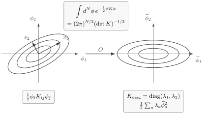
A quadratic form $\frac12\phi_iK_{ij}\phi_j$ becomes a product of independent one-dimensional Gaussians after rotating to eigenmodes $\widetilde\phi_a$. The determinant factor is the product $\prod_a\lambda_a^{-1/2}=(\det K)^{-1/2}$.

Now add a source $J_i$:

$$Z_0[J] =\int d^N\phi\, \exp\left(-\frac12\phi_iK_{ij}\phi_j+J_i\phi_i\right).$$

Complete the square. Define

$$\phi_i=\chi_i+(K^{-1})_{ij}J_j.$$

Then

$$-\frac12\phi K\phi+J\phi =-\frac12\chi K\chi+\frac12 J_i(K^{-1})_{ij}J_j,$$

so

$$\boxed{ Z_0[J]=Z_0[0]\, \exp\left(\frac12J_i(K^{-1})_{ij}J_j\right). }$$

Every Gaussian correlator follows by differentiating this expression with respect to $J$ and then setting $J=0$:

$$\langle \phi_{i_1}\cdots\phi_{i_n}\rangle =\left.\frac{1}{Z_0[0]} \frac{\partial}{\partial J_{i_1}}\cdots \frac{\partial}{\partial J_{i_n}}Z_0[J]\right|_{J=0}.$$

The two-point function is

$$\boxed{ \langle \phi_i\phi_j\rangle=(K^{-1})_{ij}. }$$

This is the finite-dimensional version of the statement that the propagator is the inverse of the quadratic operator. In a Gaussian calculation the same operator $K$ therefore plays three distinct roles: it appears in the exponent, its inverse gives correlations, and its determinant gives the normalization. Keeping those roles separate prevents many later mistakes.

Wick theorem from the Gaussian

Since $Z_0[J]$ is the exponential of a quadratic form in $J$, each nonzero derivative at $J=0$ must pair the derivatives. Odd moments vanish,

$$\langle\phi_{i_1}\cdots\phi_{i_{2n+1}}\rangle=0,$$

and even moments are sums over complete pairings:

$$\boxed{ \langle\phi_{i_1}\cdots\phi_{i_{2n}}\rangle = \sum_{\text{pairings }P} \prod_{(a,b)\in P}(K^{-1})_{i_a i_b}. }$$

For four variables this gives

$$\begin{aligned} \langle\phi_i\phi_j\phi_k\phi_\ell\rangle ={}&(K^{-1})_{ij}(K^{-1})_{k\ell} +(K^{-1})_{ik}(K^{-1})_{j\ell} \\ &+(K^{-1})_{i\ell}(K^{-1})_{jk}. \end{aligned}$$

Nothing specifically quantum has entered yet. Wick theorem is a theorem about Gaussian measures. The quantum content enters when the Gaussian variables are the values of a field or coordinate at different times, and the matrix $K^{-1}$ is the time-ordered Green function selected by the boundary condition.

A useful way to remember the counting is this. To pair $2n$ labels, choose a partner for the first label in $2n-1$ ways, then pair the remaining $2n-2$ labels. Therefore the number of terms is

$$(2n-1)!!=(2n-1)(2n-3)\cdots3\cdot1.$$

This is exactly the number that appeared in the operator proof of Wick theorem.

Integration by parts and the inverse operator

There is a second way to see why the inverse matrix appears. Gaussian integration by parts says that the integral of a total derivative vanishes:

$$0=\int d^N\phi\, \frac{\partial}{\partial\phi_i}\left(F(\phi)e^{-S[\phi]}\right), \qquad S[\phi]=\frac12\phi_aK_{ab}\phi_b.$$

Expanding the derivative gives

$$\left\langle\frac{\partial F}{\partial\phi_i}\right\rangle = \left\langle F\frac{\partial S}{\partial\phi_i}\right\rangle =K_{ij}\langle F\phi_j\rangle.$$

For $F(\phi)=\phi_k$, this becomes

$$\delta_{ik}=K_{ij}\langle\phi_j\phi_k\rangle.$$

Therefore

$$\langle\phi_j\phi_k\rangle=(K^{-1})_{jk}.$$

For a product $F=\phi_{i_1}\cdots\phi_{i_n}$, the same identity gives the recursion

$$K_{ij}\langle\phi_j\phi_{i_1}\cdots\phi_{i_n}\rangle = \sum_{a=1}^n\delta_{i i_a} \langle\phi_{i_1}\cdots\widehat{\phi_{i_a}}\cdots\phi_{i_n}\rangle.$$

Multiplying by $K^{-1}$ gives

$$\boxed{ \langle\phi_i\phi_{i_1}\cdots\phi_{i_n}\rangle = \sum_{a=1}^n(K^{-1})_{i i_a} \langle\phi_{i_1}\cdots\widehat{\phi_{i_a}}\cdots\phi_{i_n}\rangle. }$$

This recursion is Wick theorem in one line. It is also the finite-dimensional ancestor of Schwinger–Dyson identities. In a field theory, the ordinary derivative $\partial/\partial\phi_i$ is replaced by a functional derivative $\delta/\delta\phi(x)$, and the matrix $K$ is replaced by a differential operator such as $\Box+m^2$.

From many integrals to a path integral

The path integral should be read first as a limiting prescription, not as a mysterious new measure. One discretizes time, integrates over the intermediate coordinates, and only then lets the time step go to zero.

Now replace the finite list of variables $\phi_i$ by the values of a coordinate $q(t)$ at many time slices. Let

$$t_j=t_i+j\epsilon, \qquad j=0,1,\ldots,N, \qquad \epsilon=\frac{t_f-t_i}{N},$$

and fix the endpoints

$$q_0=q_i, \qquad q_N=q_f.$$

For a particle with Lagrangian

$$L(q,\dot q)=\frac{m}{2}\dot q^2-V(q),$$

the time-sliced action is approximated by

$$S_\epsilon[q] =\sum_{j=0}^{N-1}\epsilon\left[ \frac{m}{2}\left(\frac{q_{j+1}-q_j}{\epsilon}\right)^2 -V(q_j) \right].$$

The Dirac–Feynman prescription is then

$$\boxed{ \mathcal K(q_f,t_f;q_i,t_i) =\int_{q(t_i)=q_i}^{q(t_f)=q_f}\mathcal Dq\,e^{iS[q]}. }$$

More explicitly,

$$\mathcal K(q_f,t_f;q_i,t_i) =\lim_{N\to\infty}\mathcal N_N \int\prod_{j=1}^{N-1}dq_j\, \exp\left(iS_\epsilon[q]\right),$$

where $\mathcal N_N$ is fixed by the short-time normalization and composition law. For the free particle one may choose

$$\mathcal N_N=\left(\frac{m}{2\pi i\epsilon}\right)^{N/2}.$$

The notation $\mathcal Dq$ hides this limiting procedure. It is not an ordinary Lebesgue measure on a space of smooth paths. It is a shorthand for the limit of many ordinary integrals.

This point matters in practice. If one only wants normalized correlation functions, many overall constants cancel. If one wants transition amplitudes, determinants, vacuum energies, anomalies, or finite-temperature partition functions, the normalization of the measure is part of the physics and cannot be ignored.

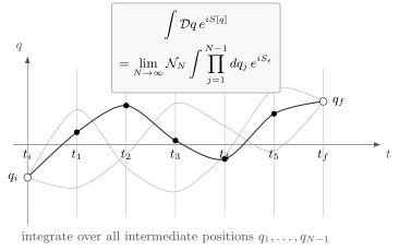
A path integral is defined by inserting many intermediate positions $q_1,\ldots,q_{N-1}$ between fixed endpoints. The continuum notation $\mathcal Dq$ is shorthand for the limit of these ordinary integrations.

The short-time factor behind this construction is the free-particle kernel

$$K_\epsilon(q_{j+1};q_j) =\left(\frac{m}{2\pi i\epsilon}\right)^{1/2} \exp\left[\frac{im}{2\epsilon}(q_{j+1}-q_j)^2\right],$$

with the potential contributing approximately $e^{-i\epsilon V(q_j)}$. Multiplying these short-time amplitudes and integrating over intermediate positions gives the full transition amplitude.

Classical paths as stationary phase

The word “classical” here does not mean “ignore fluctuations.” It means that the phase changes least rapidly near paths that solve the classical boundary-value problem. Quantum mechanics then integrates over fluctuations around those paths.

Restore $\hbar$ for a moment. The real-time weight is

$$e^{iS[q]/\hbar}.$$

When $\hbar$ is small compared with the variation of the action, nearby histories generally have rapidly changing phases and cancel. The exception is a path $q_{\mathrm{cl}}(t)$ for which the first variation vanishes:

$$\left.\frac{\delta S}{\delta q(t)}\right|_{q=q_{\mathrm{cl}}}=0.$$

This is the Euler–Lagrange equation. For

$$S[q]=\int_{t_i}^{t_f}dt\left(\frac{m}{2}\dot q^2-V(q)\right),$$

fixed endpoints imply $\delta q(t_i)=\delta q(t_f)=0$, and

$$\delta S =\int_{t_i}^{t_f}dt\, \left(-m\ddot q-V'(q)\right)\delta q.$$

Thus the stationary path obeys

$$\boxed{ m\ddot q_{\mathrm{cl}}(t)+V'(q_{\mathrm{cl}}(t))=0. }$$

Now write

$$q(t)=q_{\mathrm{cl}}(t)+\eta(t), \qquad \eta(t_i)=\eta(t_f)=0.$$

Expanding the action gives

$$S[q]=S[q_{\mathrm{cl}}] +\frac12\int dt\,dt'\,\eta(t)K(t,t')\eta(t')+\text{higher terms},$$

where

$$K(t,t')=\left[-m\frac{d^2}{dt^2}-V''(q_{\mathrm{cl}}(t))\right]\delta(t-t')$$

for this one-dimensional mechanical problem. The linear term is absent because $q_{\mathrm{cl}}$ is stationary. Therefore, at quadratic order,

$$\mathcal K(q_f,t_f;q_i,t_i) \approx \mathcal C(\hbar)\,e^{iS[q_{\mathrm{cl}}]/\hbar} \left[\det_{\mathrm D}(K+i0)\right]^{-1/2},$$

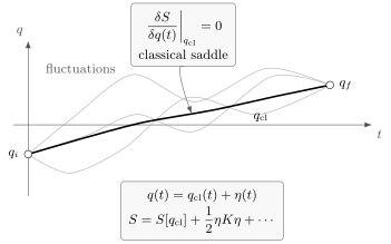
where $\det_{\mathrm D}$ is the determinant on fluctuations satisfying the Dirichlet conditions $\eta(t_i)=\eta(t_f)=0$. The measure-dependent power of $\hbar$ is included in $\mathcal C(\hbar)$, while the $i0$ prescription fixes the phase of the oscillatory determinant. This formula is the stationary-phase version of the finite-dimensional Gaussian determinant.

The classical trajectory is the stationary point of the action among paths with fixed endpoints. Writing $q=q_{\mathrm{cl}}+\eta$, the first variation vanishes and the leading quantum correction is the Gaussian integral over fluctuations $\eta$.

For a free particle, the classical path is the straight line

$$q_{\mathrm{cl}}(t)=q_i+\frac{t-t_i}{T}(q_f-q_i), \qquad T=t_f-t_i,$$

and the classical action is

$$S[q_{\mathrm{cl}}]=\frac{m(q_f-q_i)^2}{2T}.$$

The exact kernel is

$$\mathcal K(q_f,t_f;q_i,t_i) =\left(\frac{m}{2\pi i\hbar T}\right)^{1/2} \exp\left[\frac{im(q_f-q_i)^2}{2\hbar T}\right].$$

For a free theory, the stationary-phase answer is exact because the action has no higher powers of the fluctuation. This is the same reason that Wick theorem is exact for a Gaussian theory.

From this point onward we return to the course convention $\hbar=1$.

Correlators as path-integral averages

The endpoint kernel $\mathcal K(q_f,t_f;q_i,t_i)$ and the vacuum correlators used in QFT are not the same object. The kernel fixes initial and final positions. Vacuum correlators instead project the endpoints onto the ground state by the same small imaginary-time tilt that produced the Feynman prescription. With that vacuum boundary condition selected by $i\epsilon$, the path integral computes time-ordered expectation values:

$$\boxed{ \langle0|\mathcal T q(t_1)\cdots q(t_n)|0\rangle = \frac{\int\mathcal Dq\,e^{iS[q]}q(t_1)\cdots q(t_n)} {\int\mathcal Dq\,e^{iS[q]}}. }$$

For a quadratic action this is the continuum version of the finite-dimensional Gaussian average, with one Lorentzian difference: because the weight is $e^{iS}$ rather than $e^{-S}$, the time-ordered two-point function carries an extra factor of $i$ relative to the bare inverse of the quadratic kernel. If

$$S[q]=\frac12\int dt\,dt'\,q(t)K(t,t')q(t'),$$

then the real-time Feynman two-point function obeys

$$\int dt'\,K(t,t')G_F(t',t'')=i\delta(t-t'')$$

with the boundary condition fixed by the $i\epsilon$ prescription.

For the harmonic oscillator in real time,

$$K(t,t')=-(\partial_t^2+\omega^2)\delta(t-t'),$$

and the Feynman Green function is

$$G_F(t-t')=\int\frac{dE}{2\pi}\, \frac{i\,e^{-iE(t-t')}}{E^2-\omega^2+i\epsilon}.$$

It follows that

$$(\partial_t^2+\omega^2)G_F(t-t')=-i\delta(t-t').$$

The four-point function is then the Gaussian Wick sum

$$\begin{aligned} &\langle0|\mathcal T q(t_1)q(t_2)q(t_3)q(t_4)|0\rangle \\ &\quad= G_F(t_1-t_2)G_F(t_3-t_4) +G_F(t_1-t_3)G_F(t_2-t_4) \\ &\qquad +G_F(t_1-t_4)G_F(t_2-t_3). \end{aligned}$$

This is the same pairing formula as before, now expressed as an integral over histories.

From quantum mechanics to fields

Field theory is obtained by replacing the single coordinate $q(t)$ with a field $\phi(\mathbf x,t)$. A path in quantum mechanics is a function of time. A path in field theory is a whole spacetime field configuration.

For a free scalar field, the action is quadratic:

$$S_0[\phi]=\frac12\int d^4x\,\phi(x)K\phi(x),$$

where, in the Lorentzian conventions of this course,

$$K=-(\Box+m^2)$$

up to integrations by parts and the $i\epsilon$ prescription. The field-theory Gaussian integral has the formal structure

$$Z_0[0]=\int\mathcal D\phi\,e^{iS_0[\phi]} \propto (\det K)^{-1/2},$$

and the propagator is the inverse of $K$:

$$K_xG_F(x-y)=i\delta^{(4)}(x-y)$$

with signs depending on where the factor of $i$ is placed in the definition of $K$. Equivalently, using the convention stated in the course overview,

$$(\Box_x+m^2)G_F(x-y)=-i\delta^{(4)}(x-y).$$

This is the continuum analogue of

$$K_{ij}\langle\phi_j\phi_k\rangle=\delta_{ik}.$$

The formal determinant and inverse operator are the two outputs of every free path integral. The determinant contributes vacuum diagrams and normalization factors. The inverse operator gives the propagator lines used in Wick contractions.

Summary

Gaussian integration is the algebraic skeleton of free quantum field theory. A quadratic form $K$ gives two pieces of data: $(\det K)^{-1/2}$ from the normalization, and $K^{-1}$ from the two-point function. All higher Gaussian moments are sums over pairings of $K^{-1}$, which is Wick theorem.

The path integral is the continuum version of the same construction. A quantum amplitude is obtained by integrating $e^{iS}$ over histories. In the classical limit the integral is organized by stationary phase, so the dominant histories are fluctuations around solutions of $\delta S=0$. If the action is quadratic, the expansion around the classical path terminates and the Gaussian result is exact.

For quantum field theory, the variables are field values $\phi(x)$ rather than particle positions $q(t)$. The quadratic operator in the action is inverted to obtain the Feynman propagator. Interactions will be introduced by adding non-quadratic terms and expanding them as insertions in this Gaussian measure.

Common pitfalls

Do not confuse the determinant with the propagator. The determinant comes from integrating over fluctuations with no external insertions; the propagator comes from inserting two fields or differentiating twice with respect to a source.

Do not treat $\mathcal Dq$ or $\mathcal D\phi$ as an ordinary finite-dimensional measure. It is a compact notation for a limiting procedure, and its normalization matters when absolute transition amplitudes or determinants are needed.

The real-time path integral is not convergent in the ordinary sense. The symbol $e^{iS}$ needs an $i\epsilon$ prescription, a Wick rotation, or a specified contour. Without that extra information, the inverse operator is ambiguous. A Euclidean Gaussian has a positive quadratic form; a Lorentzian Gaussian has a boundary condition.

Stationary phase does not mean that only the classical path contributes. It means that the integral is organized around the classical path. The Gaussian fluctuations give the leading quantum correction, and interactions among fluctuations give higher corrections.

Do not read the Lorentzian path integral as an ordinary probability measure. The weights are phases. Probabilistic intuition becomes reliable only after a Wick rotation to a convergent Euclidean integral or after forming physical probabilities from amplitudes.

For a quadratic action, Wick theorem is exact. For a non-quadratic action, Wick theorem applies only after expanding the interaction and evaluating each term with the quadratic Gaussian measure.

Do not identify $K^{-1}$ with the Feynman propagator until the signature and source convention are fixed. In Euclidean signature the covariance is literally the inverse of a positive operator. In Lorentzian signature, with the conventions of this course, the two-point function is $i$ times the inverse of the quadratic operator with the Feynman boundary condition.

Exercises

Exercise 1: One-dimensional Gaussian moments

Evaluate

$$I[J]=\int_{-\infty}^{\infty}d\phi\, \exp\left(-\frac12a\phi^2+J\phi\right), \qquad a>0,$$

and use it to compute $\langle\phi^2\rangle$ and $\langle\phi^4\rangle$.

Solution

Complete the square:

$$-\frac12a\phi^2+J\phi =-\frac12a\left(\phi-\frac{J}{a}\right)^2+\frac{J^2}{2a}.$$

Therefore

$$I[J]=\sqrt{\frac{2\pi}{a}}\exp\left(\frac{J^2}{2a}\right).$$

The normalized moments are

$$\langle\phi^n\rangle =\left.\frac{1}{I[0]}\frac{d^nI[J]}{dJ^n}\right|_{J=0}.$$

Thus

$$\langle\phi^2\rangle=\frac1a,$$

and

$$\langle\phi^4\rangle=3\frac{1}{a^2}.$$

The factor $3$ is the number of pairings of four identical insertions.

Exercise 2: Inverse matrix from integration by parts

Let

$$Z_0[0]=\int d^N\phi\,e^{-\frac12\phi_iK_{ij}\phi_j}$$

with $K$ symmetric and positive. Show, using integration by parts rather than a source, that

$$\langle\phi_i\phi_j\rangle=(K^{-1})_{ij}.$$

Solution

Use

$$0=\int d^N\phi\,\frac{\partial}{\partial\phi_a} \left(\phi_j e^{-\frac12\phi K\phi}\right).$$

Expanding the derivative gives

$$0=\int d^N\phi\, \left(\delta_{aj}-\phi_jK_{ab}\phi_b\right)e^{-\frac12\phi K\phi}.$$

Divide by $Z_0[0]$:

$$\delta_{aj}=K_{ab}\langle\phi_b\phi_j\rangle.$$

Multiplying by $(K^{-1})_{ia}$ gives

$$\langle\phi_i\phi_j\rangle=(K^{-1})_{ij}.$$

Exercise 3: Free-particle classical path

Use the free-particle action

$$S[q]=\int_{t_i}^{t_f}dt\,\frac{m}{2}\dot q^2$$

with endpoints $q(t_i)=q_i$ and $q(t_f)=q_f$ to find the classical path and its action.

Solution

The Euler–Lagrange equation is

$$m\ddot q=0.$$

Thus the classical path is linear:

$$q_{\mathrm{cl}}(t)=A+Bt.$$

Writing $T=t_f-t_i$ and imposing the endpoints gives

$$q_{\mathrm{cl}}(t)=q_i+\frac{t-t_i}{T}(q_f-q_i).$$

The velocity is constant:

$$\dot q_{\mathrm{cl}}=\frac{q_f-q_i}{T}.$$

Therefore

$$S[q_{\mathrm{cl}}] =\int_{t_i}^{t_f}dt\,\frac{m}{2}\left(\frac{q_f-q_i}{T}\right)^2 =\frac{m(q_f-q_i)^2}{2T}.$$

Exercise 4: Harmonic-oscillator classical path

For the harmonic oscillator

$$S[q]=\int_{0}^{T}dt\left(\frac12\dot q^2-\frac12\omega^2q^2\right),$$

show that the classical path with $q(0)=q_i$ and $q(T)=q_f$ is

$$q_{\mathrm{cl}}(t)= \frac{q_f\sin\omega t+q_i\sin\omega(T-t)}{\sin\omega T},$$

assuming $\sin\omega T\ne0$.

Solution

The equation of motion is

$$\ddot q+\omega^2q=0.$$

The general solution is

$$q(t)=A\cos\omega t+B\sin\omega t.$$

The condition $q(0)=q_i$ gives $A=q_i$. The condition $q(T)=q_f$ gives

$$q_f=q_i\cos\omega T+B\sin\omega T,$$

so

$$B=\frac{q_f-q_i\cos\omega T}{\sin\omega T}.$$

Therefore

$$q_{\mathrm{cl}}(t)=q_i\cos\omega t +\frac{q_f-q_i\cos\omega T}{\sin\omega T}\sin\omega t.$$

Using

$$\sin\omega(T-t)=\sin\omega T\cos\omega t-\cos\omega T\sin\omega t,$$

this becomes

$$q_{\mathrm{cl}}(t)= \frac{q_f\sin\omega t+q_i\sin\omega(T-t)}{\sin\omega T}.$$

Exercise 5: Euclidean continuum Gaussian recursion

For a convergent Euclidean quadratic path integral with weight $e^{-S_E}$ and positive kernel $K_E(t,t')$, show that the Gaussian recursion

$$\int dt'\,K_E(t,t')\langle q(t')q(t_1)\cdots q(t_n)\rangle_E = \sum_{a=1}^n\delta(t-t_a) \langle q(t_1)\cdots\widehat{q(t_a)}\cdots q(t_n)\rangle_E$$

is the continuum analogue of the finite-dimensional integration-by-parts identity.

Solution

The finite-dimensional Euclidean identity is

$$K_{ij}\langle\phi_j\phi_{i_1}\cdots\phi_{i_n}\rangle = \sum_{a=1}^n\delta_{i i_a} \langle\phi_{i_1}\cdots\widehat{\phi_{i_a}}\cdots\phi_{i_n}\rangle.$$

To pass to the continuum, replace the discrete label $i$ by time $t$, replace the sum over $j$ by an integral over $t'$, replace $K_{ij}$ by $K_E(t,t')$, and replace the Kronecker delta by the Dirac delta:

$$\sum_j K_{ij}\phi_j \longrightarrow \int dt'\,K_E(t,t')q(t'), \qquad \delta_{i i_a}\longrightarrow\delta(t-t_a).$$

This gives

$$\int dt'\,K_E(t,t')\langle q(t')q(t_1)\cdots q(t_n)\rangle_E = \sum_{a=1}^n\delta(t-t_a) \langle q(t_1)\cdots\widehat{q(t_a)}\cdots q(t_n)\rangle_E.$$

The identity is the Euclidean Gaussian Schwinger–Dyson equation. For $n=1$ it says that the Euclidean two-point function is the inverse of $K_E$. In Lorentzian signature with weight $e^{iS}$ and $\hbar=1$, the same integration-by-parts step instead gives

$$\int dt'\,K(t,t')\langle q(t')q(t_1)\cdots q(t_n)\rangle =i\sum_{a=1}^n\delta(t-t_a) \langle q(t_1)\cdots\widehat{q(t_a)}\cdots q(t_n)\rangle,$$

so the $n=1$ case agrees with $KG_F=i\delta$ in the main text.

References and further reading

• Mark Srednicki, Quantum Field Theory, Sections 6–8, for path integrals in quantum mechanics, the harmonic oscillator, and free scalar field theory with sources.
• Sidney Coleman, Lectures of Sidney Coleman on Quantum Field Theory, Chapters 4 and 28, for the operator-to-path-integral viewpoint and functional integration.
• A. Zee, Quantum Field Theory in a Nutshell, Chapter I.2 and Appendix A, for the physical path-integral picture and Gaussian identities.
• Steven Weinberg, The Quantum Theory of Fields, Volume I, Chapter 9 and Appendix A, for path-integral methods and Gaussian multiple integrals.