Order–Disorder Duality and Ising Fermions

The two-dimensional Ising model contains a fermionic variable even though its microscopic spins are ordinary commuting numbers. The variable is a point-split product of an order field and a neighboring disorder field. Its sign under a full turn comes from order–disorder monodromy, and an elementary identity for one Ising bond gives it an exact first-order lattice propagation law.

This page derives that statement at lattice spacing $a>0$. It does not yet take the relativistic continuum limit or write the continuum Majorana equation; those are the next lesson’s subjects. Keeping this boundary sharp lets us see exactly which fermionic properties follow from topology and which require a scaling limit.

Required background. Disorder lines, branch cuts, and defect operators proves path independence and the sign acquired when a disorder line crosses a spin insertion. Kramers–Wannier duality supplies the dual-coupling relation.

Helpful background. Ising graphical expansions derives the high-temperature and domain-wall sums used to interpret the dual correlators.

Kramers–Wannier exchange of order and disorder

Take a finite connected patch $\Lambda$ of the square lattice, at zero magnetic field, with isotropic coupling $K>0$ and free boundary spins. Its dual graph $\Lambda^*$ includes the exterior face as a dual site, whose spin is fixed to $+1$. These are the matched planar boundaries used in the finite-volume duality formula. The original partition function is

$$\begin{gathered} Z(K)=\sum_{\{\sigma\}} \exp\!\left(K\sum_{\langle ij\rangle}\sigma_i\sigma_j\right),\\ \sigma_i=\pm1. \end{gathered}$$

The dual coupling is defined by

$$\begin{gathered} e^{-2K^*}=\tanh K,\\ \sinh 2K\,\sinh 2K^*=1. \end{gathered}$$

The high-temperature expansion is

$$Z(K)=2^{N_s}(\cosh K)^{N_b} \sum_{C:\,\partial C=0}(\tanh K)^{|C|}.$$

With spin insertions at distinct interior sites $x$ and $y$, the parity constraint is odd at those two sites and even everywhere else. Here $\partial C$ is the set of odd-degree vertices, with addition modulo two:

$$\langle\sigma_x\sigma_y\rangle_K = {\displaystyle \sum_{C:\,\partial C=x+y}(\tanh K)^{|C|} \over \displaystyle \sum_{C:\,\partial C=0}(\tanh K)^{|C|}}.$$

The numerator contains an open high-temperature graph from $x$ to $y$, together with any number of closed components. Under duality, the same weight becomes

$$(\tanh K)^{|C|}=e^{-2K^*|C|},$$

the low-temperature weight of an unsatisfied dual bond. To identify the whole numerator, choose a reference path $\Gamma$ on original edges from $x$ to $y$, and reverse the sign of every dual coupling crossed by $\Gamma$. Write the resulting partition function as $Z^{+,*}_\Gamma(K^*)$, where $+$ fixes the exterior dual spin.

For each dual-spin configuration, let $C$ consist of the original edges crossing unsatisfied dual bonds, including those with reversed couplings. Without a seam, $\partial C=0$; with the seam, $\partial C=x+y$. Fixing the exterior spin makes this correspondence one-to-one. In both cases a configuration has weight $e^{K^*N_b}e^{-2K^*|C|}$, so the common factor cancels in the ratio:

$$\begin{aligned} \langle\sigma_x\sigma_y\rangle_{\Lambda,K} &=\frac{Z^{+,*}_\Gamma(K^*)}{Z^{+,*}(K^*)}\\ &=\langle\mu_x\mu_y\rangle_{\Lambda^*,K^*}. \end{aligned}$$

The subscripts $x,y$ on these disorder fields denote the same original vertices: they are faces of the dual model, not dual spin sites. Reversing the roles of the two models exchanges disorder with order, with the corresponding boundary conditions. On a torus the winding sectors must also be transformed; this planar equation cannot be applied to one periodic sector unchanged. The figure distinguishes a graph being summed from a seam that defines the dual ensemble.

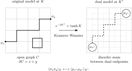
For zero field and matched planar boundaries (free original spins, fixed exterior dual spin), $t=\tanh K=e^{-2K^*}$ makes the spin-correlation graph sum equal to the dual partition ratio. The upper panel shows one allowed graph; the lower panel shows a reference seam $\Gamma$ defining reversed dual bonds. Its endpoints $x,y$ are disorder locations of the dual model. The schematic patch omits the exterior; the seam is fixed while the graphs are summed.

There is no extra local factor between the direct disorder ratio and Kadanoff–Ceva’s symmetric normalization. Their normalized partition function is

$$Y(\{K_e\})=2^{-N_s/2}Z(\{K_e\}) \prod_e[\cosh(2K_e)]^{-1/2}.$$

Every factor is unchanged by a seam reversal $K_e\mapsto-K_e$, so $Y_\Gamma/Y=Z_\Gamma/Z$ exactly. This cancellation and the order–disorder exchange are given in Kadanoff and Ceva 1971, §§ II B–C, pp. 3920–3921, Eqs. (2.7)–(2.8) and (2.14)–(2.18). A renormalized continuum twist field can be assigned a different overall normalization, but that is a separate choice from this lattice definition.

The self-dual coupling obeys $K_c=K_c^*$, so

$$\begin{gathered} \sinh 2K_c=1, \qquad \cosh 2K_c=\sqrt2,\\ K_c={1\over2}\log(1+\sqrt2). \end{gathered}$$

For the infinite zero-field square lattice this self-dual point is the critical point, using the uniqueness of the transition as in the previous duality lesson. Duality then exchanges the critical order and disorder fields, forcing equal scaling dimensions. Their value, $\Delta_\sigma=\Delta_\mu=1/8$, is additional exact critical data, not a consequence of self-duality alone; the Ising Kac table gives the continuum result $h_\sigma=\bar h_\sigma=1/16$.

The sign in a mixed correlator

A mixed correlator needs a choice of disorder cuts. Introduce the abbreviations

$$\begin{aligned} \mathcal O_\sigma&=\prod_{j=1}^n\sigma_{x_j},\\ \mathcal O_\mu&=\prod_{b=1}^{2m}\mu(p_b^*). \end{aligned}$$

If $\Gamma'$ is obtained by sweeping $\Gamma$ across a contractible region $R$ while preserving the boundary data and endpoints, the previous lesson proved

$$\begin{aligned} \left\langle\mathcal O_\sigma\mathcal O_\mu\right\rangle_{\Gamma'} &=(-1)^{N_R}\\ &\quad\times \left\langle\mathcal O_\sigma\mathcal O_\mu\right\rangle_\Gamma, \end{aligned}$$

where $N_R$ counts spin insertions in $R$ modulo $2$. Thus transporting a cut around one order insertion gives a minus sign. In continuum notation for the same monodromy,

$$\boxed{ \sigma(e^{2\pi i}z)\mu(0) =-\sigma(z)\mu(0). }$$

This is the monodromy of a square root. It does not mean that the microscopic numbers $\sigma_i$ and $\mu_{p^*}$ literally anticommute. Rather, mixed correlators live on a double cover of the configuration space of insertion points.

The same distinction matters when two order–disorder composites are exchanged. With cuts transported consistently, the exchange path has one order–cut crossing and the continued correlator changes sign. An operator anticommutation relation can be built from this rule after an ordering and cut convention is chosen, but the primary lattice statement is the sign under cut transport.

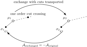
Exchanging two point-split composites while transporting their cuts produces one order–disorder crossing. The analytically continued amplitude is therefore the negative of the original amplitude.

Corner fields and antiperiodicity

Let $x$ be an original-lattice site and let the four neighboring dual sites be $x+e_a$, with

$$\begin{aligned} e_1&={a\over2}(1,1), & e_2&={a\over2}(-1,1),\\ e_3&={a\over2}(-1,-1), & e_4&={a\over2}(1,-1). \end{aligned}$$

Indices are cyclic in the geometry, $e_{a+4}=e_a$, but a cut convention must also be transported. Define the point-split fields

$$\chi_a(x)=\sigma_x\mu_{x+e_a}, \qquad a=1,2,3,4.$$

Each $\chi_a$ sits at a corner between a primal site and a dual site. The label $a$ is a local frame direction, not an internal flavor.

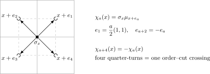
The corner field $\chi_a(x)=\sigma_x\mu_{x+e_a}$ remembers the direction $e_a$ of the point splitting and the way its disorder cut leaves the insertion.

Advance $a$ through four quarter-turns while transporting the cut. The disorder endpoint returns to the same dual site, but it has gone once around $\sigma_x$. The cut therefore crosses the order insertion once, and

$$\boxed{ \chi_{a+4}(x)=-\chi_a(x). }$$

This rules out the scalar rule $\chi_{a+4}=\chi_a$. Label a corner-frame harmonic by its phase $e^{is\alpha}$ under advancing the frame by $\alpha$, with the cut transported. A full turn gives

$$e^{2\pi i s}=-1,$$

so $s\in\frac12+\mathbb Z$. The corner field is spinorial because its local frame is antiperiodic. At finite lattice spacing only quarter-turns are lattice symmetries. This frame operation at fixed $x$ must be distinguished from the active rotation of a continuum field and its argument, whose convention is derived in the next lesson.

Choose continuously lifted corner angles $\theta_a=\pi/4+(a-1)\pi/2$, so $\theta_{a+4}=\theta_a+2\pi$. Reducing these angles separately to principal arguments would lose the sign of a half-angle after passing the branch cut. The real antiperiodic components can be projected onto definite quarter-turn harmonics,

$$\begin{gathered} u_s(x)={1\over4}\sum_{a=1}^4 e^{-is\theta_a}\chi_a(x),\\ s=\pm{1\over2},\ \pm{3\over2}. \end{gathered}$$

Equivalent formulations attach half-angle phases directly to the corners. Such phase conventions change the appearance of the difference equations but not their spectrum or the $2\pi$ sign.

The exact local propagation relation

Move the disorder endpoint from $x+e_a$ to $x+e_{a+1}$. The dual step crosses the original-lattice bond from $x$ to

$$x+\delta_a, \qquad \delta_a=e_a+e_{a+1}.$$

Explicitly,

$$\begin{aligned} \delta_1&=a(0,1), & \delta_2&=a(-1,0),\\ \delta_3&=a(0,-1), & \delta_4&=a(1,0). \end{aligned}$$

Choose the local cuts so that the configuration on the left differs from the one after the move by the crossed-bond factor

$$e^{-2K\sigma_x\sigma_{x+\delta_a}} =\cosh 2K-(\sinh 2K) \sigma_x\sigma_{x+\delta_a}.$$

Multiply by the spin already present in $\chi_a$. Since $\sigma_x^2=1$,

$$\begin{aligned} &\sigma_x e^{-2K\sigma_x\sigma_{x+\delta_a}}\\ &\qquad=\cosh 2K\,\sigma_x -\sinh 2K\,\sigma_{x+\delta_a}. \end{aligned}$$

The disorder endpoint after the move is $x+e_{a+1}$. Relative to the neighboring spin site,

$$x+e_{a+1} =(x+\delta_a)+e_{a+2},$$

because $e_{a+1}-\delta_a=-e_a=e_{a+2}$. Thus the two terms are exactly the corner fields $\chi_{a+1}(x)$ and $\chi_{a+2}(x+\delta_a)$. Inside a correlator, away from coincident additional insertions and with the other cuts kept outside this local move,

$$\boxed{ \begin{aligned} \chi_a(x) &=\cosh 2K\,\chi_{a+1}(x)\\ &\quad-\sinh 2K\,\chi_{a+2}(x+\delta_a). \end{aligned} }$$

Here $a\in\mathbb Z$, with the antiperiodic extension $\chi_{a+4}=-\chi_a$. This correlator identity is written with the spectator insertions suppressed. When another insertion meets the local move, contact terms must be included; the homogeneous equation alone does not determine the coincident correlator. See Polyakov 1987, § 10.3.1, pp. 276–278, Eqs. (10.58)–(10.61) and the discussion after (10.69). His unit-spacing bond vector $\delta_{a+1}$ is the vector called $\delta_a$ here.

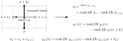
For $a=1$, moving the dual endpoint from $e_1$ to $e_2$ crosses the north bond $\delta_1=e_1+e_2$. The elementary bond identity transfers the spin from $x$ to $x+\delta_1$, producing the three-term propagation law.

This is a first-order difference equation because a single local move relates neighboring spinor components and neighboring sites. It is an exact lattice propagation equation; no continuum approximation has been made.

Critical spin-one-half modes

The antiperiodicity diagonalizes the internal quarter-turn. For a slowly varying mode, write

$$\chi_a(x)=e^{iqa}u(x).$$

The condition $\chi_{a+4}=-\chi_a$ requires

$$\begin{gathered} e^{4iq}=-1,\\ q\in\left\{ {\pi\over4},-{\pi\over4}, {3\pi\over4},-{3\pi\over4} \right\}\pmod{2\pi}. \end{gathered}$$

Because one increment of $a$ is a physical rotation by $\pi/2$, these four phases correspond to spins

$$s={2q\over\pi} \in\left\{ {1\over2},-{1\over2},{3\over2},-{3\over2}\right\}\pmod{4}.$$

First ignore spatial variation, so $u(x+\delta_a)=u(x)$. The propagation equation becomes

$$D(q,K)u=0,$$

with

$$\begin{aligned} D(q,K) &=1-\cosh(2K)e^{iq}\\ &\quad+\sinh(2K)e^{2iq}. \end{aligned}$$

For $q=\pm\pi/4$, this kernel vanishes precisely at

$$\cosh 2K=\sqrt2, \qquad \sinh 2K=1,$$

which is the self-dual coupling $K_c$. The $q=\pm3\pi/4$ pair remains nonzero there. Thus the critical lattice equation singles out the spin-$\pm\frac12$ sector, as in Polyakov 1987, § 10.3.1, p. 277, Eqs. (10.62)–(10.66).

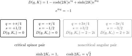
Antiperiodicity allows four quarter-turn harmonics. At $K_c$, $D(q,K_c)=0$ for $q=\pm\pi/4$, the spin-$\pm\frac12$ pair, while the spin-$\pm\frac32$ pair stays noncritical.

Restoring the slow spatial variation expands

$$u(x+\delta_a) =u(x)+\delta_a^i\partial_i u(x)+O(a^2).$$

The zeroth-order term vanishes in the critical spin-$\frac12$ sector, leaving a first-order derivative operator. Away from $K_c$, the nonzero zeroth-order remainder becomes a mass term. Deriving the resulting two-dimensional Majorana equation, including its rotation representation and continuum normalization, belongs to the next lesson.

What the lattice construction proves

It is useful to separate three claims:

1. Exact topology: order–disorder continuation around one endpoint gives $-1$.
2. Exact lattice dynamics: the bond identity gives the three-term propagation relation.
3. Continuum identification: the long-wavelength spin-$\pm\frac12$ modes become the two components of a Majorana field.

The first two have been proved here at finite lattice spacing. The third requires the scaling-limit analysis that follows. In particular, the microscopic spins have not been turned into Grassmann numbers; fermionic statistics are encoded in the cut-dependent operator algebra and its analytic continuation.

Common pitfalls

Dropping the cut data. The product $\sigma_x\mu_{x+e_a}$ is not specified by its two endpoints alone. Its sign depends on how the disorder cut is continued.

Using $\chi_{a+4}=\chi_a$. Returning the endpoint geometrically is not the same as transporting the cut around the spin. The correct continuation is antiperiodic.

Calling any four-point linear relation discrete holomorphicity. The exact statement here is the propagation equation derived from one bond. Discrete holomorphic or s-holomorphic formulations require specified projections and phase conventions.

Claiming a continuum Majorana equation too early. The critical kernel identifies spin-$\frac12$ zero modes, but spatial Taylor expansion and field normalization are still needed.

Exercises

Exercise 1: the self-dual coupling

Starting from $e^{-2K^*}=\tanh K$, derive

$$\sinh 2K\,\sinh 2K^*=1$$

and solve for $K_c=K_c^*$.

Solution

Let $x=e^{-2K^*}=\tanh K$. Then

$$\begin{aligned} \sinh 2K^* &={x^{-1}-x\over2}\\ &={1-\tanh^2K\over2\tanh K}\\ &={1\over\sinh 2K}. \end{aligned}$$

At self-duality, $\sinh^2 2K_c=1$. Since $K_c>0$,

$$\sinh 2K_c=1, \qquad e^{2K_c}=1+\sqrt2,$$

and therefore

$$K_c={1\over2}\log(1+\sqrt2).$$

Exercise 2: why a full turn gives a minus sign

Transport $x+e_a$ through $e_{a+1},e_{a+2},e_{a+3},e_{a+4}=e_a$ while keeping $\sigma_x$ fixed. Use the disorder-line deformation rule to show $\chi_{a+4}(x)=-\chi_a(x)$.

Solution

The four local moves carry the disorder endpoint once around the order insertion. The initial and final endpoints agree, but the transported cut differs from the initial cut by a small closed loop surrounding $x$. Removing that loop requires flipping the spin in its interior. Since the correlator contains one $\sigma_x$, the variable change contributes $-1$. Hence $\chi_{a+4}=-\chi_a$.

Exercise 3: derive the propagation law for $a=1$

Take $e_1=\frac a2(1,1)$ and $e_2=\frac a2(-1,1)$. Show that moving the dual endpoint from $x+e_1$ to $x+e_2$ crosses the bond from $x$ to $x+a(0,1)$, and derive

$$\begin{aligned} \chi_1(x) &=\cosh 2K\,\chi_2(x)\\ &\quad-\sinh 2K\,\chi_3(x+a\hat y). \end{aligned}$$

Solution

The dual step crosses the north bond, so $\delta_1=e_1+e_2=a\hat y$. Its weight ratio is

$$e^{-2K\sigma_x\sigma_{x+a\hat y}} =\cosh2K-\sinh2K\,\sigma_x\sigma_{x+a\hat y}.$$

Multiplying by $\sigma_x$ gives a first term with spin at $x$ and a second with spin at $x+a\hat y$. After the move, the disorder endpoint is $x+e_2$. Relative to $x+a\hat y$, it lies at

$$x+e_2-(x+a\hat y) =-{a\over2}(1,1)=e_3.$$

The two terms are therefore $\chi_2(x)$ and $\chi_3(x+a\hat y)$, with the stated coefficients.

Exercise 4: allowed angular harmonics

Solve $e^{4iq}=-1$ and convert each $q$ into Euclidean spin $s=2q/\pi$. Why are there exactly four modes modulo $2\pi$?

Solution

The solutions are

$$q={\pi\over4}+{n\pi\over2}, \qquad n=0,1,2,3,$$

modulo $2\pi$. They may be represented as $q=\pm\pi/4,\pm3\pi/4$. Since a unit change of $a$ is a rotation by $\pi/2$, $e^{iq}=e^{is\pi/2}$ and $s=2q/\pi$. This gives $s=\pm1/2,\pm3/2$ modulo $4$. Four corner components give four independent Fourier modes.

Exercise 5: the critical zero modes

Evaluate

$$D(q,K)=1-\cosh(2K)e^{iq}+\sinh(2K)e^{2iq}$$

for $q=\pm\pi/4$ and show that $D=0$ requires $\sinh 2K=1$. Check that $q=\pm3\pi/4$ are not zero modes at that coupling.

Solution

For $q=\pi/4$,

$$D=1-{\cosh2K\over\sqrt2}(1+i)+i\sinh2K.$$

The real part vanishes when $\cosh2K=\sqrt2$. The imaginary part then vanishes when $\sinh2K=1$. These conditions are compatible because $\cosh^2x-\sinh^2x=1$. The $q=-\pi/4$ equation is the complex conjugate.

At $q=3\pi/4$ and $K=K_c$,

$$D=1-(-1+i)-i=2-2i\ne0,$$

while the $q=-3\pi/4$ value is its complex conjugate. Thus only the spin-$\pm1/2$ pair is critical.

References

• L. P. Kadanoff and H. Ceva, “Determination of an Operator Algebra for the Two-Dimensional Ising Model,” Physical Review B 3, 3918–3939 (1971), doi:10.1103/PhysRevB.3.3918.
• A. M. Polyakov, Gauge Fields and Strings. Contemporary Concepts in Physics, Vol. 3. Harwood Academic Publishers, 1987, § 10.3.1, doi:10.1201/9780203755082.

Further reading

• D. Chelkak and S. Smirnov, “Universality in the 2D Ising Model and Conformal Invariance of Fermionic Observables,” Inventiones Mathematicae 189, 515–580 (2012), doi:10.1007/s00222-011-0371-2.
• P. Di Francesco, P. Mathieu, and D. Sénéchal, Conformal Field Theory. Graduate Texts in Contemporary Physics. Springer, 1997, Chapters 4 and 12.
• B. M. McCoy and T. T. Wu, The Two-Dimensional Ising Model. Harvard University Press, 1973.
• T. D. Schultz, D. C. Mattis, and E. H. Lieb, “Two-Dimensional Ising Model as a Soluble Problem of Many Fermions,” Reviews of Modern Physics 36, 856–871 (1964), doi:10.1103/RevModPhys.36.856.