Hubbard–Stratonovich Transformation and the Continuum Field

The previous page used two complementary languages for the Ising model. Kramers–Wannier duality rewrote a spin system in terms of domain walls on a dual lattice, while mean-field theory replaced the fluctuating environment of a spin by an average molecular field. This page turns that mean-field idea into an exact identity.

The key move is the Hubbard–Stratonovich transformation. Instead of summing directly over spins coupled to spins, we introduce an auxiliary real variable $\phi_i$ at each lattice site. The original two-spin interaction is traded for a Gaussian action for $\phi$ plus a local coupling between $\phi_i$ and $\sigma_i$. After the spins are summed, the partition function becomes a lattice field integral:

$$Z=\int \mathcal D\phi\,e^{-S_{\mathrm{eff}}[\phi]}.$$

This is the first place in the course where a continuum field theory emerges in a precise way from a microscopic statistical system. The field $\phi$ is not guessed; it is introduced by an exact Gaussian identity. Its saddle point reproduces mean-field theory, its quadratic fluctuations give the mean-field susceptibility, and its local nonlinearities lead to the familiar Ising-universality scalar theory

$$S_E[\varphi] =\int d^d x\, \left[ {1\over2}(\partial\varphi)^2+{1\over2}r\varphi^2+{u\over4!}\varphi^4+\cdots \right].$$

The dots are not decoration. They remind us that the lattice produces infinitely many local operators. Near a critical point, the renormalization group decides which of them remain important.

Required background. Kramers–Wannier duality and mean-field theory supplies the Ising normalization, the molecular-field equation, and the Gaussian critical point used below.

Gaussian contraction as an operator

The Gaussian contour

We write a general ferromagnetic Ising interaction in matrix notation,

$$Z=\sum_{\{\sigma\}} \exp\left({1\over2}\sum_{i,j}K_{ij}\sigma_i\sigma_j\right), \qquad \sigma_i=\pm1,$$

where $K_{ij}=\beta J_{ij}=K_{ji}$. For the nearest-neighbor model on a hypercubic lattice,

$$K_{ij}=K A_{ij}, \qquad K=\beta J,$$

with $A_{ij}=1$ for nearest neighbors and $0$ otherwise. The factor $1/2$ prevents double counting.

The real Gaussian formula below requires $K$ to be positive definite. The unshifted nearest-neighbor adjacency matrix is not: its Fourier eigenvalues have both signs and can include zeros. For that example, the identity is understood eigenmode by eigenmode by analytic continuation, with the contour of each negative eigenmode rotated to a direction on which the Gaussian converges and any zero eigenvalue defined as a nonsingular limit. The ferromagnetic soft mode near $p=0$ remains on a real contour.

One can instead make the integral real by replacing $K$ with $K+\kappa I$ and multiplying the result by $e^{-\kappa N_s/2}$, since $\sigma_i^2=1$. That replacement is exact for the full integral, but a saddle-point or polynomial truncation depends on the chosen diagonal shift. We therefore keep the original kernel when quoting the Weiss saddle and the Gaussian susceptibility. Probabilistic statements about the auxiliary field apply directly only when the integration contour is real and positive; the algebraic identities continue analytically to the other case.

Before introducing the auxiliary field, it is useful to isolate the algebraic mechanism behind it. Let $K$ be a symmetric positive matrix and define

$$\partial K\partial = \sum_{i,j}K_{ij}{\partial^2\over\partial \phi_i\partial\phi_j}.$$

For any polynomial $F(\phi)$,

$$\boxed{ \left. \exp\left({1\over2}\partial K\partial\right)F(\phi) \right|_{\phi=0} = {\int d^N\eta\, \exp\left[-{1\over2}\eta K^{-1}\eta\right]F(\eta) \over \int d^N\eta\, \exp\left[-{1\over2}\eta K^{-1}\eta\right]} .}$$

This identity says that the exponential of a second-order differential operator performs Gaussian Wick contractions. For example,

$$\left. \exp\left({1\over2}\partial K\partial\right) \phi_i\phi_j \right|_{\phi=0} =K_{ij},$$

and

$$\left. \exp\left({1\over2}\partial K\partial\right) \phi_i\phi_j\phi_k\phi_l \right|_{\phi=0} =K_{ij}K_{kl}+K_{ik}K_{jl}+K_{il}K_{jk}.$$

The proof is just the Gaussian generating function. Introduce a source $J_i$ and compute

$${\int d^N\eta\, \exp\left[-{1\over2}\eta K^{-1}\eta+J\eta\right] \over \int d^N\eta\, \exp\left[-{1\over2}\eta K^{-1}\eta\right]} = \exp\left({1\over2}J K J\right).$$

Differentiating with respect to $J$ generates Gaussian moments. On the other hand,

$$\left. \exp\left({1\over2}\partial K\partial\right)e^{J\phi} \right|_{\phi=0} = \exp\left({1\over2}J K J\right),$$

because

$${1\over2}\partial K\partial\,e^{J\phi} ={1\over2}J K J\,e^{J\phi}.$$

The two linear functionals agree on exponentials and hence on polynomials. This is a convenient way to remember the whole Hubbard–Stratonovich construction: a spin interaction is a Gaussian contraction operator in disguise.

The Ising partition function can be represented by such an operator. Since

$$\prod_i 2\cosh \phi_i =\sum_{\{\sigma\}}e^{\sum_i\phi_i\sigma_i},$$

we have

$$\left. \exp\left({1\over2}\partial K\partial\right) \prod_i 2\cosh\phi_i \right|_{\phi=0} =\sum_{\{\sigma\}} \exp\left({1\over2}\sigma K\sigma\right) =Z.$$

Spin insertions are generated by differentiating the local factors. For instance, for distinct sites,

$$\langle \sigma_{i_1}\cdots\sigma_{i_n}\rangle ={1\over Z} \left. \exp\left({1\over2}\partial K\partial\right) \left[ \partial_{i_1}\cdots\partial_{i_n} \prod_j 2\cosh\phi_j \right] \right|_{\phi=0}.$$

This formula is exact, but it is still somewhat formal. The next step is to rewrite the contraction operator as an actual field integral.

Hubbard–Stratonovich decoupling

For a real symmetric positive-definite matrix $K$, the finite-dimensional Gaussian identity is

$$\boxed{ \exp\left({1\over2}\sigma K\sigma\right) = {1\over(2\pi)^{N/2}(\det K)^{1/2}} \int d^N\phi\, \exp\left[-{1\over2}\phi K^{-1}\phi+\phi\sigma\right]. }$$

Here

$$\phi K^{-1}\phi=\sum_{i,j}\phi_i(K^{-1})_{ij}\phi_j, \qquad \phi\sigma=\sum_i\phi_i\sigma_i.$$

To prove the identity, complete the square:

$$-{1\over2}\phi K^{-1}\phi+\phi\sigma = -{1\over2}(\phi-K\sigma)K^{-1}(\phi-K\sigma) +{1\over2}\sigma K\sigma.$$

The shifted Gaussian integrates to the normalization factor. The one-variable identity is the starting point of Hubbard 1959, p. 77, Eq. (2), PDF; diagonalizing positive $K$ gives the matrix version above. Substituting this identity into the Ising partition function gives

$$Z =\mathcal N_K \int d^N\phi\, \exp\left[-{1\over2}\phi K^{-1}\phi\right] \sum_{\{\sigma\}} \exp\left(\sum_i\phi_i\sigma_i\right),$$

where $\mathcal N_K=[(2\pi)^N\det K]^{-1/2}$. The spin sum now factorizes site by site:

$$\sum_{\{\sigma\}}e^{\sum_i\phi_i\sigma_i} =\prod_i\sum_{\sigma_i=\pm1}e^{\phi_i\sigma_i} =\prod_i 2\cosh\phi_i.$$

Thus

$$\boxed{ Z =\mathcal N_K \int d^N\phi\, \exp\left[-S_{\mathrm{eff}}(\phi)\right], }$$

with

$$\boxed{ S_{\mathrm{eff}}(\phi) ={1\over2}\sum_{i,j}\phi_i(K^{-1})_{ij}\phi_j -\sum_i\log(2\cosh\phi_i). }$$

The original spins have disappeared. Their discreteness survives in the non-polynomial local potential $-\log(2\cosh\phi)$.

For an indefinite lattice kernel, the same displayed formulas hold with the mode contours prescribed by analytic continuation. In that case $S_{\mathrm{eff}}$ is not a real probability action on $\mathbb R^{N_s}$; it is an exact contour-integral representation. This distinction is ultraviolet bookkeeping, but it must be kept separate from the later long-distance approximation.

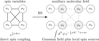
The Hubbard–Stratonovich transformation replaces a direct spin–spin interaction by an auxiliary field $\phi$. Its Gaussian quadratic kernel is $K^{-1}$, and it couples locally to the spins. After summing the spins, one obtains a lattice field theory with action $S_{\mathrm{eff}}[\phi]$.

On a real positive Gaussian contour, $\phi_i$ is a fluctuating molecular field. At fixed $\phi$, the spins are independent, and

$$\langle \sigma_i\rangle_{\phi}=\tanh\phi_i.$$

This is why $\log\cosh\phi_i$ appears: it is the one-site free energy in an external field $\phi_i$.

Saddle point and molecular field

The exact field integral is usually not easier than the original spin sum. Its advantage is conceptual: it separates local nonlinear spin physics from spatial propagation. The saddle-point equation is

$${\partial S_{\mathrm{eff}}\over\partial\phi_i}=0.$$

Since

$${\partial\over\partial\phi_i} \left({1\over2}\phi K^{-1}\phi\right) =\sum_j(K^{-1})_{ij}\phi_j,$$

and

$${d\over d\phi_i}\log(2\cosh\phi_i)=\tanh\phi_i,$$

we obtain

$$\boxed{ \sum_j(K^{-1})_{ij}\phi_j=\tanh\phi_i. }$$

Equivalently,

$$\boxed{ \phi_i=\sum_jK_{ij}\tanh\phi_j. }$$

If we define the local magnetization at the saddle by

$$m_i=\tanh\phi_i,$$

then

$$\phi_i=\sum_jK_{ij}m_j, \qquad m_i=\tanh\left(\sum_jK_{ij}m_j\right).$$

This is exactly the inhomogeneous mean-field equation. Evaluating the Hubbard–Stratonovich integral at its saddle reproduces the Weiss approximation; the integral itself remains exact. The distinction between the auxiliary-field representation and its saddle evaluation is explicit in Hubbard 1959, pp. 77–78, Eqs. (4)–(9), PDF.

For a translation-invariant ferromagnet, a uniform saddle obeys

$$\phi=K(0)\tanh\phi,$$

where

$$K(0)=\sum_j K_{ij}.$$

For a nearest-neighbor hypercubic lattice in $d$ dimensions,

$$K(0)=2dK=zK.$$

Thus the uniform saddle equation becomes

$$\phi=zK\tanh\phi.$$

Writing $m=\tanh\phi$, this is equivalent to

$$m=\tanh(zKm),$$

which is the zero-field mean-field equation from the previous page.

The saddle-point instability occurs when the linearized equation develops a nonzero solution. For small $\phi$,

$$\tanh\phi=\phi-{\phi^3\over3}+O(\phi^5).$$

The linearized equation is

$$\phi=K(0)\phi.$$

Therefore the mean-field critical point is

$$K(0)=1.$$

For the nearest-neighbor hypercubic model this gives

$$K_c^{\mathrm{MF}}={1\over 2d}.$$

This is not the exact critical point in low dimensions. In the two-dimensional square-lattice model, the exact result is $\sinh(2K_c)=1$, while mean field gives $K_c^{\mathrm{MF}}=1/4$. The discrepancy is precisely the effect of fluctuations neglected by the saddle point.

Exact correlation identities

The auxiliary field is not identical to the spin. It is a smeared molecular field. The distinction matters, and it is a common source of wrong factors.

When the Gaussian contour is real, the completed square gives a particularly transparent probabilistic derivation:

$$-{1\over2}\phi K^{-1}\phi+\phi\sigma = -{1\over2}(\phi-K\sigma)K^{-1}(\phi-K\sigma) +{1\over2}\sigma K\sigma,$$

at fixed spin configuration $\sigma$, the auxiliary field is Gaussian with

$$\mathbb E(\phi_i\mid\sigma)=\sum_jK_{ij}\sigma_j, \qquad \operatorname{Cov}(\phi_i, \phi_j\mid\sigma)=K_{ij}.$$

Averaging over spins gives the exact identities

$$\boxed{ \langle \phi_i\rangle =\sum_jK_{ij}\langle\sigma_j\rangle. }$$

For connected two-point functions,

$$\boxed{ \langle \phi_i\phi_j\rangle_c =K_{ij} +\sum_{k,l}K_{ik}K_{jl}\langle\sigma_k\sigma_l\rangle_c. }$$

Similarly,

$$\boxed{ \langle \phi_i\sigma_j\rangle_c =\sum_kK_{ik}\langle\sigma_k\sigma_j\rangle_c. }$$

In a translation-invariant system, Fourier transformation diagonalizes these relations. If

$$G_\phi(p)=\langle\phi(p)\phi(-p)\rangle_c, \qquad G_\sigma(p)=\langle\sigma(p)\sigma(-p)\rangle_c,$$

then

$$\boxed{ G_\phi(p)=K(p)+K(p)^2G_\sigma(p). }$$

Equivalently,

$$\boxed{ G_\sigma(p)={G_\phi(p)-K(p)\over K(p)^2}. }$$

Thus the pole structure of $G_\phi$ and $G_\sigma$ is the same whenever $K(p)$ is smooth and nonzero near the critical momentum. The auxiliary field carries the same long-distance critical singularity as the spin field, but its short-distance normalization is different.

There is also a useful conditional-spin identity. On a real contour, at fixed $\phi$ the spins are independent with

$$P(\sigma_i\mid\phi_i)={e^{\phi_i\sigma_i}\over2\cosh\phi_i},$$

so for distinct sites

$$\langle\sigma_i\sigma_j\rangle =\langle\tanh\phi_i\tanh\phi_j\rangle_{\phi}.$$

This formula is exact for $i\ne j$. At coincident points, the spin identity $\sigma_i^2=1$ must be handled separately. Both correlation identities extend to admissible complex contours by analyticity, although the word “conditional” then loses its probabilistic meaning.

Small-field expansion

The quadratic instability occurs in a slowly varying mode, and the saddle order parameter is small near a continuous mean-field transition. These facts motivate a local field expansion,

$$\log(2\cosh\phi) =\log2+{\phi^2\over2}-{\phi^4\over12}+{\phi^6\over45}+O(\phi^8).$$

Therefore, up to an irrelevant additive constant,

$$S_{\mathrm{eff}}(\phi) ={1\over2}\phi(K^{-1}-I)\phi +{1\over12}\sum_i\phi_i^4 -{1\over45}\sum_i\phi_i^6+O(\phi^8).$$

The quartic term is positive in the action. This is the first sign of the stable Landau potential. The alternating Taylor series is only local—the negative $\phi^6$ coefficient does not make the exact action unstable—and the higher terms are fixed by the microscopic two-state nature of the spin. Below four dimensions, small field is not by itself a controlled expansion at criticality; the renormalization group supplies the missing criterion.

For a translation-invariant lattice, define

$$\phi_i={1\over\sqrt{N_s}}\sum_p e^{ip\cdot x_i}\phi(p),$$

and

$$K(p)=\sum_j K_{ij}e^{ip\cdot(x_j-x_i)}.$$

Then the quadratic action is

$$S_2={1\over2}\sum_p \left({1\over K(p)}-1\right) \phi(p)\phi(-p).$$

The Gaussian auxiliary-field propagator is therefore

$$\boxed{ G_{\phi}^{(0)}(p) =\langle\phi(p)\phi(-p)\rangle_0 ={K(p)\over1-K(p)}. }$$

This is the random-phase or Gaussian mean-field susceptibility in auxiliary-field variables. Using the exact relation between $G_\phi$ and $G_\sigma$, the corresponding spin susceptibility is

$$G_{\sigma}^{(0)}(p) ={1\over1-K(p)}.$$

The denominator tells us where the Gaussian theory becomes massless: its instability occurs when the maximum eigenvalue of $K(p)$ reaches $1$. This is the mean-field critical condition; interactions can shift the actual transition.

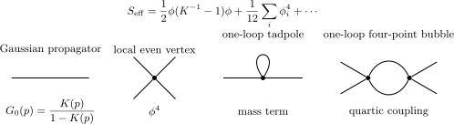
Expanding $\log\cosh\phi$ gives a Gaussian propagator $G_0(p)=K(p)/(1-K(p))$ and local even vertices. The one-loop tadpole corrects the quadratic term, while the one-loop four-point bubble corrects the quartic coupling; these are field-theory loops, not occupied-bond graphs.

The diagrammatic language here is different from the high-temperature loop expansion. In the high-temperature expansion, graphs are occupied bonds of the original lattice. Here, diagrams are perturbative contractions of a continuum or lattice scalar field. The two languages are related by universality, not by term-by-term equality.

Continuum limit

Take a translation-invariant ferromagnet with finite-range or exponentially decaying couplings on a lattice of spacing $a$. Its interaction kernel is analytic near its maximum at $p=0$. Assume also that the quadratic gradient term is isotropic and nondegenerate, as for equal couplings along all axes of a hypercubic lattice. Then

$$K(p)=K_0-\rho p^2+O(p^4), \qquad K_0=K(0), \qquad \rho>0.$$

The quadratic kernel becomes

$${1\over K(p)}-1 = \left({1\over K_0}-1\right) +{\rho\over K_0^2}p^2+O(p^4).$$

Translation invariance alone does not imply this isotropy. For example, unequal square-lattice couplings give $K(p)=2K_x\cos(ap_x)+2K_y\cos(ap_y)$, with quadratic coefficients $K_xa^2$ and $K_ya^2$. In that case one keeps a positive tensor $\rho_{ab}p_ap_b$ or explicitly rescales the spatial coordinates. A vanishing stiffness in some direction requires a different long-distance expansion.

Keeping the finite-lattice Fourier normalization used above, the quadratic action at small momentum is

$$S_2 \approx {1\over2}\sum_p \left(r_0+c_0p^2\right)\phi(p)\phi(-p),$$

where

$$r_0={1\over K_0}-1, \qquad c_0={\rho\over K_0^2}.$$

To pass to physical position space, let $x_i=ai$, let the periodic box have volume $V=N_sa^d$, and define the slowly varying interpolation by $\phi(x_i)=\phi_i$. The lattice field is dimensionless. A site sum becomes

$$\sum_i F(\phi_i) \simeq {1\over a^d}\int_V d^d x\,F(\phi(x)).$$

For a periodic interpolation supported on the retained Fourier modes, Parseval’s identity gives

$$\begin{aligned} \sum_p\phi(p)\phi(-p)&={1\over a^d}\int_V d^d x\,\phi(x)^2,\\ \sum_p p^2\phi(p)\phi(-p)&={1\over a^d}\int_V d^d x\,(\nabla\phi)^2. \end{aligned}$$

Thus the same cell-volume factor multiplies the quadratic terms. To the displayed derivative order,

$$S_2 \approx {1\over a^d}\int_V d^d x\, \left[ {c_0\over2}(\nabla\phi)^2+{r_0\over2}\phi^2 \right].$$

The quartic term becomes local:

$${1\over12}\sum_i\phi_i^4 \longrightarrow {1\over12a^d}\int_V d^d x\,\phi(x)^4.$$

The factor $a^{-d}$ occurs in both terms because the same unrescaled interpolation $\phi(x)$ is used. In mass dimensions, $[r_0]=0$ and $[c_0]=-2$. Define the canonically normalized field and its matched coefficients by

$$\varphi=\sqrt{c_0\over a^d}\,\phi, \qquad r={r_0\over c_0}, \qquad u={2a^d\over c_0^2}.$$

Then $[\varphi]=(d-2)/2$, $[r]=2$ and $[u]=4-d$. The resulting action is

$$\boxed{ S_E[\varphi] =\int d^d x\, \left[ {1\over2}(\partial\varphi)^2+{1\over2}r\varphi^2+{u\over4!}\varphi^4+ \sum_{n\ge3}g_{2n}\varphi^{2n} +\sum_{m\ge2}c_m\varphi(-\nabla^2)^m\varphi+ \cdots \right]. }$$

The field $\varphi$ is the continuum representative of the Ising spin operator. More precisely, it is any coarse-grained scalar field with the same long-distance singularity and the same $\mathbb Z_2$ transformation law. The microscopic normalization is not universal.

Check the field matching. For a constant lattice field $\phi_i=A$, the two retained local terms are $N_sr_0A^2/2$ and $N_sA^4/12$. Substituting $V=N_sa^d$ and $\varphi=\sqrt{c_0/a^d}\,A$ gives

$${Vr\varphi^2\over2}={N_sr_0A^2\over2}, \qquad {Vu\varphi^4\over4!}={N_sA^4\over12}.$$

Both terms agree for arbitrary $a$, not only in lattice units $a=1$. These are coefficients matched at the microscopic cutoff within the small-momentum expansion. Integrating out further modes changes them; the bare condition $r=0$ does not locate the exact interacting critical surface.

In the following figure, the lattice and continuum fields therefore have different normalizations. Inspect the change from the dimensionless site variable $\phi_i$ to the field $\varphi$ with a canonical kinetic term.

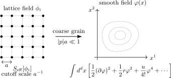
The dimensionless site field $\phi_i$ is interpolated as $\phi(x_i)$ and normalized as $\varphi=\sqrt{c_0/a^d}\,\phi$. For $|p|a\ll1$ and positive isotropic stiffness, the gradient expansion gives the displayed local scalar action. Its coefficients can run when more modes are integrated out. The diagram is schematic and not to scale.

The continuum action is an effective field theory with a cutoff of order $a^{-1}$. It is not a literal classical field theory valid at arbitrarily high momentum. The lattice spacing prevents the ultraviolet catastrophe that a classical continuum thermal field would otherwise have. The renormalization group will later explain how universal long-distance quantities can become insensitive to the details of that cutoff.

Example: nearest-neighbor hypercubic lattice

For the nearest-neighbor Ising model in $d$ dimensions,

$$K_{ij}=K A_{ij},$$

where $A_{ij}=1$ if $i$ and $j$ are nearest neighbors. The Fourier transform is

$$K(p)=2K\sum_{\mu=1}^d\cos(p_\mu a).$$

This is the unshifted physical interaction kernel. Its negative ultraviolet eigenvalues require the analytically continued HS contours described above, but the critical ferromagnetic mode is the maximum at $p=0$ and has a real Gaussian direction.

At small momentum,

$$\cos(p_\mu a)=1-{a^2p_\mu^2\over2}+O(p^4a^4),$$

so

$$K(p)=2dK-Ka^2p^2+O(p^4a^4).$$

The Gaussian spin susceptibility is

$$G_\sigma^{(0)}(p) ={1\over1-2K\sum_\mu\cos(p_\mu a)}.$$

At small $p$,

$$G_\sigma^{(0)}(p) \approx {1\over(1-2dK)+Ka^2p^2}.$$

This has the Ornstein–Zernike form

$$G(p)\sim {1\over r_\sigma+c_\sigma p^2},$$

with

$$r_\sigma=1-2dK, \qquad c_\sigma=Ka^2.$$

These coefficients belong to the dimensionless lattice spin susceptibility; $r_\sigma$ is not the dimension-two coefficient $r$ of the canonically normalized action.

The Gaussian second-moment correlation length of the spin field is therefore

$$\xi^2={c_\sigma\over r_\sigma} ={Ka^2\over1-2dK}.$$

As $K\nearrow K_c^{\mathrm{MF}}=1/(2d)$,

$$\xi\sim |K-K_c^{\mathrm{MF}}|^{-1/2}.$$

The exponent $1/2$ is the mean-field value. Near this Gaussian critical point the exponential decay length has the same leading divergence; at a finite distance from criticality it is determined by the full lattice kernel, not just its quadratic expansion. The exact critical exponents in low dimensions are changed by the loop corrections generated by the local interactions in $S_{\mathrm{eff}}$.

Why the φ⁴ theory is natural

The scalar field theory near the Ising critical point is not chosen because it is the simplest thing one can write. It is forced by three facts.

First, the order parameter is a single real scalar with a $\mathbb Z_2$ symmetry:

$$\sigma_i\mapsto-\sigma_i, \qquad \phi_i\mapsto-\phi_i, \qquad \varphi(x)\mapsto-\varphi(x).$$

Therefore only even powers of the field appear.

Second, locality of the microscopic interaction implies locality of the long-distance action. Short-range couplings generate analytic functions of momentum near $p=0$, so the continuum action is an expansion in derivatives.

Third, criticality requires tuning the temperature-like direction until the inverse correlation length vanishes. At Gaussian order this is $r=0$; fluctuations shift the critical value of the coefficient in a cutoff action. The quartic term is the leading stabilizing local nonlinearity compatible with the symmetry near this ordinary transition. Higher even powers and higher derivatives are present, but their importance depends on dimension. Power counting gives

$$[\varphi]={d-2\over2}, \qquad [u]=4-d.$$

Thus $d=4$ is the upper critical dimension of the Ising $\varphi^4$ description. Above four dimensions, the quartic interaction is irrelevant and mean-field theory becomes asymptotically correct. Below four dimensions, fluctuations change the scaling laws. This is the doorway to the Wilson–Fisher fixed point.

Summary

The Hubbard–Stratonovich transformation rewrites the Ising partition function as an exact integral over an auxiliary scalar field. The effective action is

$$S_{\mathrm{eff}}(\phi) ={1\over2}\phi K^{-1}\phi- \sum_i\log(2\cosh\phi_i).$$

Its saddle equation,

$$\phi_i=\sum_jK_{ij}\tanh\phi_j,$$

is the mean-field equation in molecular-field form. Its quadratic expansion gives the Gaussian propagator

$$G_\phi^{(0)}(p)={K(p)\over1-K(p)},$$

and the corresponding spin susceptibility

$$G_\sigma^{(0)}(p)={1\over1-K(p)}.$$

When the largest eigenvalue of $K(p)$ approaches $1$, the mass term vanishes and long wavelengths dominate. Expanding $K(p)$ at small momentum and $\log\cosh\phi$ at small field produces the continuum Ising field theory,

$$S_E=\int d^d x\, \left[ {1\over2}(\partial\varphi)^2+{1\over2}r\varphi^2+{u\over4!}\varphi^4+ \cdots \right].$$

The saddle point is mean field. The loop expansion around it is the first approximation to fluctuations. The renormalization group, introduced next, tells us when those loops are small, when they are large, and why universality survives.

Common pitfalls

Identifying the auxiliary field with the spin. The field $\phi$ is a molecular field with a different short-distance normalization. It has the same long-distance critical pole, but correlators differ by contact and kernel factors such as

$$G_\phi(p)=K(p)+K(p)^2G_\sigma(p).$$

Treating a truncated action as an exact identity. The Hubbard–Stratonovich integral is exact only with the full non-polynomial potential $-\log(2\cosh\phi)$. Truncating it to $\phi^4$ is a long-distance approximation near a continuous transition.

Ignoring the Gaussian contour. A real HS probability measure requires a positive-definite kernel. For the unshifted nearest-neighbor kernel, rotate the negative-eigenvalue contours; a diagonal shift is exact only before the saddle or polynomial truncation is made.

Discarding the cutoff. The continuum limit is not obtained by simply throwing away the lattice. The lattice supplies the ultraviolet cutoff; universality concerns the insensitivity of long-distance observables to many details of that cutoff.

Calling the Gaussian instability exact. The criterion $K(0)=1$ is a mean-field condition. In dimensions below the upper critical dimension, fluctuations shift the critical point and change the critical exponents.

Exercises

Exercise 1

Prove the finite-dimensional Hubbard–Stratonovich identity

$$\exp\left({1\over2}J K J\right) ={1\over(2\pi)^{N/2}(\det K)^{1/2}} \int d^N\phi\, \exp\left[-{1\over2}\phi K^{-1}\phi+J\phi\right]$$

for a positive-definite symmetric matrix $K$.

Solution

Complete the square:

$$-{1\over2}\phi K^{-1}\phi+J\phi =-{1\over2}(\phi-KJ)K^{-1}(\phi-KJ) +{1\over2}J K J.$$

Then shift the integration variable,

$$\eta=\phi-KJ.$$

The Jacobian is $1$, so the integral becomes

$$e^{{1\over2}J K J} {1\over(2\pi)^{N/2}(\det K)^{1/2}} \int d^N\eta\, \exp\left[-{1\over2}\eta K^{-1}\eta\right].$$

The remaining Gaussian is

$$\int d^N\eta\, \exp\left[-{1\over2}\eta K^{-1}\eta\right] =(2\pi)^{N/2}(\det K)^{1/2}.$$

The normalization cancels it, leaving

$$\exp\left({1\over2}J K J\right).$$

Taking $J_i=\sigma_i$ gives the Hubbard–Stratonovich identity used in the Ising model.

Exercise 2

Starting from

$$S_{\mathrm{eff}}(\phi) ={1\over2}\phi K^{-1}\phi-\sum_i\log(2\cosh\phi_i),$$

show that the uniform saddle-point equation on a $z$-coordinated nearest-neighbor lattice is equivalent to

$$m=\tanh(zKm).$$

Solution

The saddle equation is

$$\sum_j(K^{-1})_{ij}\phi_j=\tanh\phi_i.$$

Multiplying by $K$ gives

$$\phi_i=\sum_jK_{ij}\tanh\phi_j.$$

For a uniform saddle,

$$\phi_i=\phi, \qquad \tanh\phi_i=m.$$

For a nearest-neighbor lattice with coordination number $z$,

$$\sum_jK_{ij}=zK.$$

Therefore

$$\phi=zKm.$$

Since $m=\tanh\phi$, we find

$$m=\tanh(zKm),$$

which is the Weiss mean-field equation.

Exercise 3

For the nearest-neighbor hypercubic lattice, use

$$K(p)=2K\sum_{\mu=1}^d\cos(p_\mu a)$$

to derive the small-momentum Gaussian spin susceptibility and its second-moment correlation length on the disordered side.

Solution

The Gaussian spin susceptibility is

$$G_\sigma^{(0)}(p)={1\over1-K(p)}.$$

At small momentum,

$$\cos(p_\mu a)=1-{a^2p_\mu^2\over2}+O(p^4a^4).$$

Thus

$$K(p)=2K\sum_{\mu=1}^d\left(1-{a^2p_\mu^2\over2}+\cdots\right) =2dK-Ka^2p^2+O(p^4a^4).$$

Therefore

$$G_\sigma^{(0)}(p) \approx {1\over1-2dK+Ka^2p^2}.$$

This has the form

$$G_\sigma^{(0)}(p)\approx{1\over r_\sigma+c_\sigma p^2},$$

with

$$r_\sigma=1-2dK, \qquad c_\sigma=Ka^2.$$

The Gaussian second-moment correlation length is

$$\xi^2={c_\sigma\over r_\sigma} ={Ka^2\over1-2dK}.$$

As $K\to K_c^{\mathrm{MF}}=1/(2d)$ from below,

$$\xi\sim |K-K_c^{\mathrm{MF}}|^{-1/2}.$$

Exercise 4

Use the conditional Gaussian interpretation of the Hubbard–Stratonovich field to prove

$$\langle \phi_i\phi_j\rangle_c =K_{ij}+ \sum_{k,l}K_{ik}K_{jl}\langle\sigma_k\sigma_l\rangle_c.$$

Then show that in Fourier space this implies

$$G_\sigma(p)={G_\phi(p)-K(p)\over K(p)^2}.$$

Solution

At fixed spin configuration, completing the square shows that $\phi$ is Gaussian with mean

$$\mathbb E(\phi_i\mid\sigma)=\sum_kK_{ik}\sigma_k$$

and covariance

$$\operatorname{Cov}(\phi_i,\phi_j\mid\sigma)=K_{ij}.$$

Therefore

$$\langle\phi_i\phi_j\rangle =K_{ij}+ \left\langle \left(\sum_kK_{ik}\sigma_k\right) \left(\sum_lK_{jl}\sigma_l\right) \right\rangle.$$

Also

$$\langle\phi_i\rangle =\sum_kK_{ik}\langle\sigma_k\rangle.$$

Subtracting $\langle\phi_i\rangle\langle\phi_j\rangle$ gives

$$\langle \phi_i\phi_j\rangle_c =K_{ij}+ \sum_{k,l}K_{ik}K_{jl} \left( \langle\sigma_k\sigma_l\rangle- \langle\sigma_k\rangle\langle\sigma_l\rangle \right).$$

Hence

$$\langle \phi_i\phi_j\rangle_c =K_{ij}+ \sum_{k,l}K_{ik}K_{jl}\langle\sigma_k\sigma_l\rangle_c.$$

For a translation-invariant system, convolution becomes multiplication in momentum space:

$$G_\phi(p)=K(p)+K(p)^2G_\sigma(p).$$

Solving for $G_\sigma(p)$ gives

$$G_\sigma(p)={G_\phi(p)-K(p)\over K(p)^2}.$$

Exercise 5

Starting from

$$\log(2\cosh\phi)=\log2+{\phi^2\over2}-{\phi^4\over12}+O(\phi^6),$$

show that the long-distance effective action has a positive quartic coupling. Why is this positivity important near the mean-field critical point?

Solution

The effective action is

$$S_{\mathrm{eff}}(\phi) ={1\over2}\phi K^{-1}\phi- \sum_i\log(2\cosh\phi_i).$$

Substitute the expansion:

$$S_{\mathrm{eff}}(\phi) =\text{constant} +{1\over2}\phi K^{-1}\phi -\sum_i\left({\phi_i^2\over2}-{\phi_i^4\over12}+O(\phi_i^6)\right).$$

Thus

$$S_{\mathrm{eff}}(\phi) =\text{constant} +{1\over2}\phi(K^{-1}-I)\phi +{1\over12}\sum_i\phi_i^4 +O(\phi^6).$$

The quartic coefficient in the action is positive. Near the mean-field critical point, the quadratic coefficient of the zero-momentum mode approaches zero. If the leading nonlinear term were not stabilizing, the small-field Landau expansion would not define a stable local potential. The positive quartic term stabilizes the theory and gives the standard double-well structure when the mass term becomes negative.

References

• Hubbard, John. “Calculation of Partition Functions.” Physical Review Letters 3, no. 2 (1959): 77–78. DOI. Open PDF.

Further reading

• Goldenfeld, Nigel. Lectures on Phase Transitions and the Renormalization Group. Frontiers in Physics 85. Reading, MA: Addison-Wesley, 1992. Chapters 2–5.
• Kardar, Mehran. Statistical Physics of Fields. Cambridge: Cambridge University Press, 2007. Chapters 2–5.
• Polyakov, Alexander M. Gauge Fields and Strings. Contemporary Concepts in Physics 3. Chur: Harwood Academic Publishers, 1987. Chapters 1–3.
• Stratonovich, Ruslan L. “On a Method of Calculating Quantum Distribution Functions.” Soviet Physics Doklady 2 (1958): 416–419. English translation of the 1957 Russian original; the translation is identified in Hubbard 1959, p. 78, note 1, PDF.
• Zinn-Justin, Jean. Quantum Field Theory and Critical Phenomena. 5th ed. Oxford: Oxford University Press, 2021. Chapters 1 and 14–16.