Effective Actions, Dimensional Estimates, and IR Physics

The first lesson of advanced QFT is not a new Feynman rule. It is a change of attitude. A quantum field theory is usually not a microscopic final answer written once and for all; it is a description valid at a chosen scale. When a separation of scales permits a controlled derivative expansion, long-distance physics can be approximated by local operators of the remaining light fields, constrained by symmetries and kept through a specified order.

This viewpoint is familiar outside high-energy physics. Hydrodynamics does not know about atoms in detail, but it knows about conservation of mass, momentum, and energy. Elasticity does not know every electron wavefunction in a crystal, but it knows about displacements and strain. General relativity is the long-distance theory of a massless spin-two field, and Yang–Mills theory is the long-distance theory of massless spin-one gauge fields. In all cases the same logic appears: identify the slow variables, impose the symmetries, and organize the action by dimensional estimates.

The subtlety is that massless fields are never completely short-distance or long-distance spectators. Their loop integrals can contain infrared singularities, and marginal interactions produce logarithms rather than simple powers. Those logarithms are the first signal of renormalization-group flow, which will become the main engine of the next several pages. The practical task is therefore to identify the light degrees of freedom and symmetry-allowed operators, then keep only those that matter at the desired accuracy in $p/M$ or $a/\ell$. The next six lessons turn that power counting into explicit loop and RG calculations.

Effective actions and scale separation

Dimensions and gauge-field normalization. The symbol $D$ denotes spacetime dimension. For the engineering-dimension estimates on this page,

$$[x]=-1, \qquad [\partial_\mu]=1, \qquad [S]=0, \qquad [\mathcal L]=D.$$

The displayed Wilsonian integrals and loop estimates use Euclidean momenta. Lorentzian statements use the site-wide $(+---)$ convention.

For Yang–Mills theory we often use an anti-Hermitian geometric connection, translated explicitly from the site’s Hermitian-generator convention. Let $T^a$ be Hermitian with $\operatorname{Tr}_F(T^aT^b)=\delta^{ab}/2$, and define

$$\mathbf A=-ie_0 A_{\rm can}^aT^a, \qquad \mathbf F=d\mathbf A+\mathbf A\wedge\mathbf A =-ie_0F_{\rm can}^aT^a.$$

Use the positive invariant bilinear

$$\operatorname{tr}_{\rm geom}(XY):=-2\operatorname{Tr}_F(XY).$$

The Euclidean action is then

$$S_{\mathrm{YM}} ={1\over 4e_0^2}\int d^D x\, \operatorname{tr}_{\rm geom}(\mathbf F_{\mu\nu}\mathbf F_{\mu\nu}) ={1\over4}\int d^Dx\,F_{{\rm can},\mu\nu}^aF_{{\rm can},\mu\nu}^a\ge0.$$

Thus $[\mathbf A]=1$ and $[e_0^2]=4-D$. The relation $\mathbf A=-ie_0A_{\rm can}$ puts the kinetic term in canonical form and moves $e_0$ into the interaction vertices. Equivalently, $D=d+\mathbf A=d-ie_0A_{\rm can}$, so this is only a translated basis and normalization, not a different charge convention.

Let $a$ be a microscopic length scale. It could be a lattice spacing, an inverse heavy-particle mass, a molecular mean free path, or simply a UV cutoff scale. A long-distance experiment probes lengths

$$\ell\gg a,$$

or momenta

$$p\sim {1\over \ell}\ll \Lambda_0, \qquad \Lambda_0\sim {1\over a}.$$

A Wilsonian effective action at scale $\mu$ is defined by keeping modes with momenta below $\mu$ and integrating out modes above $\mu$, with the UV regulator, field measure and mode split fixed. Schematically, in Euclidean notation,

$$e^{-S_\mu[\Phi_<]} = \int_{\mu<|k|<\Lambda_0}\mathcal D\Phi_>\, e^{-S_{\Lambda_0}[\Phi_<+\Phi_>]}.$$

Exact blocking generally produces kernels that connect distinct points. A local derivative expansion is available only when those kernels admit a controlled expansion in external momenta much smaller than $\mu$; merely retaining $|p|<\mu$ is insufficient. In that domain, the quasi-local expansion is written as

$$S_\mu[\Phi] = \int d^D x\, \sum_i c_i(\mu)\,\mathcal O_i(x),$$

where each $\mathcal O_i$ is a local operator built from the low-energy fields and their derivatives. A finite truncation approximates the exact blocked functional rather than replacing it identically. The coefficients $c_i(\mu)$ remember the short-distance physics.

Where this expansion is controlled, it is a Taylor expansion in slow variation. If $\Phi(x)$ changes appreciably only over a distance $\ell$, each derivative costs a factor of order

$$\partial \sim {1\over \ell}.$$

When coefficients are governed by the removed short length $a$, a term with two more derivatives is suppressed by a power such as

$$\left({a\over \ell}\right)^2,$$

unless a symmetry, a massless pole, or a near-critical enhancement changes the counting. The following schematic illustrates this controlled long-wavelength expansion, not exact locality of every sharply blocked functional.

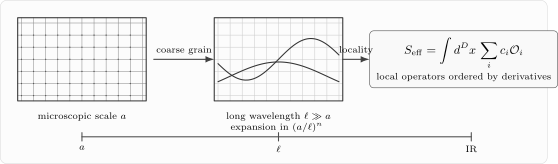
An effective action is organized by locality and symmetry. After short-distance modes at scale $a$ are removed, the remaining fields vary on a scale $\ell\gg a$, and higher-derivative terms are suppressed by powers of $a/\ell$.

There are two important qualifications.

First, the Wilsonian effective action is not the same object as the full one-particle-irreducible effective action. A Wilsonian action integrates out only a specified momentum band; its quasi-local approximation requires the domain just stated. Sharp cutoff surfaces can obstruct an analytic expansion. A suitable smooth blocking prescription can avoid that obstruction but does not by itself prove analyticity; see the regulated Wilson action and its expansion. A full 1PI effective action also integrates over soft massless fluctuations and can contain nonlocal terms such as $\log(-\Box)$ or $1/\Box$.

Second, the word “effective” does not mean “uncontrolled.” In its declared domain, a low-energy effective action can make systematically improvable predictions, organized by powers of $p/M$ for a removed scale $M$. A removed-state pole or threshold, massless nonanalyticity, or loss of scale separation can invalidate the expansion rather than merely change a coefficient.

Hydrodynamics as the prototype

Hydrodynamics is the cleanest example of effective reasoning. A fluid has complicated microscopic constituents, but its long-wavelength variables are fixed by conservation laws. For a nonrelativistic fluid, the slow variables include the mass density $\rho$, velocity $\mathbf v$, pressure $p$, and energy density.

The Euler equation is the leading derivative approximation to momentum conservation:

$$\rho\left(\partial_t v_i+v^j\partial_jv_i\right)=-\partial_i p.$$

The left-hand side is the convective acceleration of a fluid element. The right-hand side is the force density from the pressure gradient. This equation is not the most general one compatible with the symmetries. It is the leading one in a derivative expansion.

At the next order one may add viscous terms. For a parity-invariant isotropic fluid in three spatial dimensions,

$$\rho\left(\partial_t v_i+v^j\partial_jv_i\right) = -\partial_i p +\eta\nabla^2 v_i +\left(\zeta+{\eta\over3}\right)\partial_i(\partial_jv^j) +\cdots,$$

where $\eta$ is the shear viscosity and $\zeta$ is the bulk viscosity. The ellipsis denotes terms with more derivatives or more powers of fluctuations.

The hierarchy is controlled by the Knudsen number

$$\mathrm{Kn}={a\over \ell},$$

where $a$ is a microscopic relaxation length and $\ell$ is the macroscopic variation length of the flow. Viscosity is not less fundamental than pressure; it is simply less important at sufficiently long wavelengths.

A still simpler example is diffusion. Suppose $n(t,\mathbf x)$ is a conserved density. Conservation gives

$$\partial_t n+\nabla\cdot\mathbf j=0.$$

The constitutive relation is then written as the most general derivative expansion compatible with rotation invariance and the absence of a preferred direction. To first order,

$$\mathbf j=-\mathcal D\nabla n+\cdots,$$

where $\mathcal D$ is the diffusion constant. Combining the two equations gives

$$\partial_t n=\mathcal D\nabla^2 n+\cdots.$$

For a Fourier mode $n\propto e^{-i\omega t+i\mathbf k\cdot\mathbf x}$,

$$-i\omega=-\mathcal D\mathbf k^2+\cdots, \qquad \omega=-i\mathcal D\mathbf k^2+\cdots.$$

The damping rate is proportional to $\mathbf k^2$. A higher-derivative correction would produce terms such as $\mathbf k^4$. Thus the derivative expansion is directly visible in the dispersion relation.

Hydrodynamics teaches the main lesson: one does not need to solve the microscopic theory to know the structure of the long-distance theory. Symmetry and locality already do a large part of the work.

Dimensional estimates

In $D$ spacetime dimensions, the action is dimensionless:

$$[S]=0.$$

Since

$$[d^D x]=-D,$$

a Lagrangian density has dimension

$$[\mathcal L]=D.$$

If a local operator $\mathcal O$ has scaling dimension $\Delta$, and the action contains

$$S\supset \int d^Dx\,c_{\mathcal O}\mathcal O(x),$$

then

$$[c_{\mathcal O}]=D-\Delta.$$

At a momentum scale $p$, the corresponding dimensionless coupling is

$$g_{\mathcal O}(p)\sim c_{\mathcal O}\,p^{\Delta-D}.$$

This formula is the simplest power-counting form of the renormalization group. It says:

• If $\Delta<D$, then $g_{\mathcal O}(p)$ grows as $p\to0$. The operator is relevant.
• If $\Delta=D$, then $g_{\mathcal O}(p)$ is classically scale independent. The operator is marginal.
• If $\Delta>D$, then $g_{\mathcal O}(p)$ decreases as $p\to0$. The operator is irrelevant.

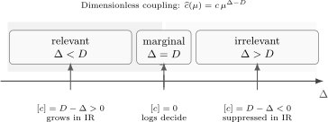
Power counting around a scale-invariant theory. The coupling dimension is $D-\Delta$. Relevant operators grow in the infrared, irrelevant operators die away, and marginal operators require loop-level information.

The language is about the infrared. “Relevant” means relevant at long distances; “irrelevant” means suppressed at long distances. The labels are not moral judgments. Irrelevant operators often encode extremely important short-distance physics, but their effects are small at low momentum.

Scalar-field warm-up

For a scalar with kinetic term

$$S_0={1\over2}\int d^Dx\,\partial_\mu\phi\,\partial_\mu\phi,$$

we have

$$2+2[\phi]=D,$$

so

$$[\phi]={D-2\over2}.$$

A monomial $\phi^n$ has engineering dimension

$$\Delta_n=n{D-2\over2},$$

and a coupling $\lambda_n\phi^n$ has

$$[\lambda_n]=D-n{D-2\over2}.$$

Thus $\phi^4$ is classically marginal in $D=4$, while $\phi^6$ is irrelevant in $D=4$. In $D=3$, $\phi^6$ is classically marginal. This is why the same operator can play different roles in different dimensions.

Heavy fields and local operators

A useful check is a conditional Gaussian elimination in Euclidean signature. Take real fields and real $g$, with $m^2\geq0$ and $M^2>0$. Use a finite periodic box and a finite UV mode cutoff so that the heavy kernel is a real symmetric positive matrix. We integrate the heavy coordinates at fixed regulated light field; this does not assume that the joint light/heavy measure is normalizable:

$$S_E[\phi,\chi] = \int d^Dx\left[ {1\over2}\phi(-\partial^2+m^2)\phi +{1\over2}\chi(-\partial^2+M^2)\chi +{g\over2}\chi\phi^2 \right].$$

For fixed $\phi$, the heavy field appears quadratically. Products and inverse kernels below are understood in the regulated heavy-mode space: if modes are truncated, the source $g\phi^2/2$ is projected onto that space. Define

$$K_\chi=-\partial^2+M^2, \qquad J={g\over2}\phi^2.$$

Then

$${1\over2}\chi K_\chi\chi+J\chi ={1\over2}(\chi+K_\chi^{-1}J)K_\chi(\chi+K_\chi^{-1}J) -{1\over2}J K_\chi^{-1}J.$$

The shifted heavy Gaussian gives a determinant independent of $\phi$ and the following exact field-dependent contribution, also obtained by classical heavy-field elimination. The determinant can be omitted for this matching calculation, but not when computing the vacuum normalization or free energy:

$$\Delta S_{\mathrm{eff}}[\phi] =-{1\over2}\int d^Dx\,d^Dy\,J(x)K_\chi^{-1}(x,y)J(y).$$

The unexpanded interaction is bilocal. For the displayed local expansion, require the unprojected source $g\phi^2/2$ to have Fourier support inside the retained heavy-mode space with $q_E^2/M^2\ll1$, so the projection leaves it unchanged. These source momenta are sums of light momenta; their sum must remain inside both bounds. Since the Euclidean inverse has denominator $M^2+q_E^2$, its low-momentum expansion is

$$K_\chi^{-1}={1\over M^2-\partial^2} ={1\over M^2}\left(1+{\partial^2\over M^2}+{\partial^4\over M^4}+\cdots\right),$$

so the local expansion begins as

$$\boxed{ \Delta\mathcal L_{E,\mathrm{eff}} =-{g^2\over8M^2}\phi^4 -{g^2\over8M^4}\phi^2\partial^2\phi^2 +O(M^{-6}). }$$

After integrating by parts with vanishing boundary term, the second term is a positive coefficient times $(\partial_\mu\phi^2)^2$. The negative induced Euclidean quartic is fixed by the displayed real interaction and positive Gaussian kernel. Each extra derivative pair is suppressed by $q_E^2/M^2$ in this domain; the series is not a uniform identity on the whole regulated field space.

The conditional integral does not establish stability: minimizing the constant heavy field leaves the potential $m^2\phi^2/2-g^2\phi^4/(8M^2)$, unbounded for nonzero real $g$. The stable Core matching example instead retains $\lambda_{\rm full}\phi^4/24$ with $\lambda_{\rm full}>3g^2/M^2$ and positive squared masses. That is a classical stability condition, not a proof of continuum quantum existence. Its induced Lorentzian Lagrangian term is positive because $\mathcal L_L$ contains minus the potential; the induced potential is negative in both signatures. Its Feynman inverse has denominator $M^2-q^2-i0$, and no finite local expansion reproduces the pole at $q^2=M^2$.

Gravity as a derivative expansion

The Einstein–Hilbert action in $D$ dimensions is

$$S_{\mathrm{EH}} ={1\over16\pi G_D}\int d^Dx\,\sqrt{|g|}\,R.$$

The scalar curvature has two derivatives of the metric,

$$R\sim \partial^2 g+g^{-1}(\partial g)(\partial g),$$

so the action begins at two-derivative order. Since $R$ has dimension $2$, Newton’s constant has dimension

$$[G_D]=2-D.$$

Equivalently, the $D$-dimensional Planck scale is defined up to conventional numerical factors by

$$M_D^{D-2}\sim {1\over G_D}.$$

To see the interaction strength, expand around flat space,

$$g_{\mu\nu}=\eta_{\mu\nu}+\kappa h_{\mu\nu}, \qquad \kappa^2\sim G_D.$$

After choosing a gauge and normalizing the kinetic term, the schematic expansion has the form

$$S_{\mathrm{EH}} \sim \int d^Dx\, \left[ (\partial h)^2 +\kappa h(\partial h)^2 +\kappa^2 h^2(\partial h)^2 +\cdots \right].$$

Each graviton vertex carries two derivatives. Thus the dimensionless gravitational expansion parameter at momentum $p$ is

$$G_Dp^{D-2}.$$

In four dimensions,

$$G_Np^2\sim {p^2\over M_{\mathrm{Pl}}^2}.$$

This is why quantum gravity is weak at low energy. It is not weak because the Einstein–Hilbert action is simple; it is weak because the coupling has negative mass dimension and therefore becomes small in the infrared.

The same estimate is visible in Newtonian language. For two particles of mass $M$ in four dimensions, the dimensionless gravitational coupling is

$$\alpha_G\sim G_NM^2\sim {M^2\over M_{\mathrm{Pl}}^2}.$$

Gravity between elementary particles is tiny when $M\ll M_{\mathrm{Pl}}$, but it becomes order one at the Planck scale.

Yang–Mills power counting

Gauge theory gives a different lesson. In the geometric normalization,

$$S_{\mathrm{YM}} ={1\over4e_0^2}\int d^Dx\, \operatorname{tr}_{\rm geom}(\mathbf F_{\mu\nu}\mathbf F_{\mu\nu}),$$

with

$$\mathbf F_{\mu\nu} =\partial_\mu\mathbf A_\nu-\partial_\nu\mathbf A_\mu +[\mathbf A_\mu,\mathbf A_\nu].$$

Here $\mathbf A_\mu$ has dimension $1$, so $\mathbf F_{\mu\nu}$ has dimension $2$. The action is dimensionless only if

$$[e_0^2]=4-D.$$

Equivalently,

$$e_0^2\sim M^{4-D}.$$

Translate back with $\mathbf A_\mu=-ie_0A_{\mu,{\rm can}}$ to put the kinetic term in canonical form. Then the schematic Lagrangian becomes

$$\mathcal L_{\mathrm{YM}} \sim (\partial A_{\rm can})^2 +e_0(\partial A_{\rm can})A_{\rm can}^2 +e_0^2A_{\rm can}^4.$$

At momentum scale $p$, the dimensionless gauge interaction is therefore

$$g_{\mathrm{eff}}^2(p)\sim e_0^2p^{D-4}.$$

This gives the classical part of the story:

$$\begin{array}{ccl} D<4 &:& g_{\mathrm{eff}}^2(p)\text{ grows in the infrared},\\ D=4 &:& g_{\mathrm{eff}}^2(p)\text{ is classically marginal},\\ D>4 &:& g_{\mathrm{eff}}^2(p)\text{ grows in the ultraviolet}. \end{array}$$

In four dimensions, ordinary power counting cannot decide whether the coupling grows or shrinks at short distances. The answer comes from logarithms. In QED the charge is screened; in non-Abelian Yang–Mills theory the gauge bosons antiscreen. The sign of the beta function is a quantum effect, not a dimensional-analysis effect.

A quick position-space estimate says the same thing. A geometric gauge potential with characteristic variation length $x$ scales as

$$\mathbf A\sim {1\over x}, \qquad \mathbf F\sim {1\over x^2}.$$

Thus the Yang–Mills action density scales like $\mathbf F^2\sim x^{-4}$. In $D=4$ this is precisely scale invariant at the classical level. Four dimensions are special because the action has no power of the overall size.

Infrared sensitivity of massless fields

Dimensional analysis is especially sharp for massless loop integrals. A typical massless two-propagator integral has the scaling form

$$I_D(p,\Lambda) \sim e_0^2\int^{\Lambda}{d^Dk\over(2\pi)^D} {1\over k^2(k+p)^2}.$$

For the purpose of power counting, the scaling region $p\ll k\ll\Lambda$ behaves like

$$I_D(p,\Lambda) \sim e_0^2\int_p^\Lambda dk\,k^{D-5}.$$

For $2<D<4$, nonzero external momentum regulates the soft regions and the integral scales as $p^{D-4}$. The radial estimate therefore gives

$$I_D(p,\Lambda) \sim \begin{cases} \displaystyle {e_0^2\over 4-D}\,p^{D-4}, & 2<D<4,\\ \displaystyle e_0^2\log{\Lambda\over p}, & D=4,\\ \displaystyle {e_0^2\over D-4}\,\Lambda^{D-4}, & D>4, \end{cases}$$

up to constants and numerator factors.

For $D\leq2$ at fixed nonzero Euclidean $p$, the neighborhoods of $k=0$ and $k=-p$ are themselves infrared divergent. Near either point the other denominator stays nonzero, leaving radial behavior $r^{D-3}dr$: logarithmically divergent at $D=2$ and worse below. A positive internal mass, or another regulator that actually controls these soft modes, is required. External Euclidean off-shellness is already present and does not cure them; neither does a UV cutoff or a finite box with an untreated zero mode. This endpoint issue is separate from the intermediate-shell estimate above.

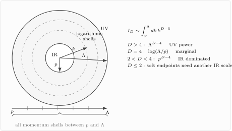
The same massless loop integral diagnoses both infrared and ultraviolet sensitivity. In four dimensions the radial estimate is logarithmic, producing the $\log(\Lambda/p)$ terms that the renormalization group will resum.

The case $D=4$ is the hinge. The integral is not dominated by a single power of the largest or smallest scale; every momentum decade contributes comparably. The resulting logarithm records the accumulation over these momentum intervals.

The phrase “IR divergence” should be used carefully. A Wilsonian effective action at scale $\mu$ integrates out only $k>\mu$, so it is protected from the deep infrared. But physical amplitudes and 1PI effective actions often integrate over all virtual momenta, including arbitrarily soft massless quanta. If the observable is sensitive to such quanta, then the result may contain singularities as $p\to0$, $m\to0$, or an energy resolution is taken to zero.

This is not a mathematical embarrassment. It is a message: the supposed low-energy observable has not included all the low-energy degrees of freedom that nature allows. Later, in gauge theory, infrared divergences will be treated by inclusive observables, Wilson lines, factorization, and effective descriptions adapted to soft and collinear modes.

Matching, running, and power counting

It is useful to separate three ideas that are often blended together.

Power counting tells us how large an operator can be at scale $p$ once its coefficient is known. It is the statement

$$g_{\mathcal O}(p)\sim c_{\mathcal O}p^{\Delta-D}.$$

Matching tells us what the coefficient $c_{\mathcal O}$ is at some reference scale. Integrating out the heavy field above, for instance, matches the coefficient of $\phi^4$ to a number proportional to $g^2/M^2$.

Running tells us how that coefficient changes as the reference scale is moved. Running is invisible in purely classical dimensional analysis; it appears when logarithmic loop integrals make many momentum decades contribute comparably.

The contact interaction on the next page isolates matching and running in a quantum-mechanical problem. The $\phi^4$ pages after that show the same logic in relativistic perturbation theory.

What the first estimates already know

The estimates above are crude, but they already know a surprising amount of physics.

They know that hydrodynamics is universal because conservation laws and symmetry fix the first terms in the derivative expansion. They know that heavy particles leave local traces suppressed by powers of their mass. They know that quantum gravity is weak at long distances and strong near the Planck scale. They know that four-dimensional gauge theory is special, because its coupling is marginal by classical power counting. They know that logarithms appear when no single scale dominates an integral.

The rest of renormalization theory refines these statements. It computes the coefficients, tracks how they depend on the sliding scale, and explains which parts are universal.

Summary

A local EFT approximates the light-field physics in a declared scale-separated domain. Its terms are constrained by symmetry and ordered by derivatives, fields, and dimensions. Exact elimination can be nonlocal, and the convergence of a conditional heavy Gaussian does not establish stability of the joint theory.

For an operator $\mathcal O$ of dimension $\Delta$ in $D$ dimensions, the coefficient $c_{\mathcal O}$ has dimension $D-\Delta$, and the dimensionless coupling at momentum $p$ is $c_{\mathcal O}p^{\Delta-D}$. This gives the basic distinction between relevant, marginal, and irrelevant operators.

Hydrodynamics is a model example of the derivative expansion: ideal-fluid terms come first, viscous terms come next, and higher-gradient terms are suppressed by powers of the microscopic length divided by the macroscopic length.

Gravity has a coupling $G_D$ with dimension $2-D$, so its quantum interactions are weak at long distances. Yang–Mills theory has $[e_0^2]=4-D$, so it is classically marginal in four dimensions. In that case quantum logarithms decide the flow.

Massless loop integrals can be infrared sensitive. In four dimensions the estimate $\int dk/k$ produces logarithms, foreshadowing the renormalization group.

Power counting, matching, and running are distinct. Power counting orders possible operators; matching fixes their coefficients at a reference scale; running tracks logarithmic dependence on that reference scale.

Common pitfalls

Mistaking an effective action for an uncontrolled approximation. A low-energy effective action is a controlled description of a specified regime. Its predictive power comes from knowing which operators matter at the desired accuracy.

Confusing Wilsonian and 1PI effective actions. The Wilsonian action admits a quasi-local approximation only when its regulated kernels have a controlled low-external-momentum expansion. The full 1PI effective action can additionally be nonlocal because arbitrarily soft massless modes have been integrated over.

Identifying “renormalizable” with “allowed.” Symmetries allow infinitely many local operators. Renormalizable operators are merely the ones that are relevant or marginal by power counting around a chosen fixed point.

Trying to remove infrared divergences with UV counterterms. UV divergences ask how short-distance physics is parametrized. IR divergences ask whether the observable is well-defined in the presence of massless long-distance quanta.

Exercises

Exercise 1

Let $\phi$ be a scalar field in $D$ spacetime dimensions with kinetic term

$$S_0={1\over2}\int d^Dx\,(\partial\phi)^2.$$

Find $[\phi]$. Then find the engineering dimension of the coupling $\lambda_n$ in

$$S_{\mathrm{int}}=\int d^Dx\,{\lambda_n\over n!}\phi^n.$$

For which $D$ is $\phi^4$ classically marginal? For which $D$ is $\phi^3$ classically marginal?

Solution

The kinetic term has dimension $D$. Since $\partial$ has dimension $1$,

$$[(\partial\phi)^2]=2+2[\phi].$$

Thus

$$2+2[\phi]=D,$$

so

$$[\phi]={D-2\over2}.$$

The operator $\phi^n$ has dimension

$$[\phi^n]=n{D-2\over2}.$$

The action is dimensionless, so

$$[\lambda_n]+n{D-2\over2}=D.$$

Therefore

$$[\lambda_n]=D-n{D-2\over2}.$$

For $\phi^4$,

$$[\lambda_4]=D-2(D-2)=4-D,$$

so $\phi^4$ is classically marginal in $D=4$.

For $\phi^3$,

$$[\lambda_3]=D-{3(D-2)\over2}=3-{D\over2},$$

so $\phi^3$ is classically marginal in $D=6$.

Exercise 2

Starting from conservation of a density $n$,

$$\partial_t n+\nabla\cdot\mathbf j=0,$$

and the leading constitutive relation

$$\mathbf j=-\mathcal D\nabla n,$$

derive the diffusion equation. Then find the dispersion relation for a mode $n(t,\mathbf x)=n_0e^{-i\omega t+i\mathbf k\cdot\mathbf x}$.

Solution

Insert the constitutive relation into the conservation law:

$$\partial_t n+\nabla\cdot(-\mathcal D\nabla n)=0.$$

For constant $\mathcal D$,

$$\partial_t n=\mathcal D\nabla^2n.$$

For a Fourier mode,

$$\partial_t n=-i\omega n, \qquad \nabla^2n=-\mathbf k^2 n.$$

The diffusion equation gives

$$-i\omega n=-\mathcal D\mathbf k^2n.$$

Hence

$$\omega=-i\mathcal D\mathbf k^2.$$

The frequency is imaginary, so the mode decays as

$$e^{-i\omega t}=e^{-\mathcal D\mathbf k^2t}.$$

The damping rate is order $\mathbf k^2$, as expected for a leading two-derivative spatial term.

Exercise 3

Use the geometric Yang–Mills normalization

$$S_{\mathrm{YM}}={1\over4e_0^2}\int d^Dx\, \operatorname{tr}_{\rm geom}(\mathbf F_{\mu\nu}\mathbf F_{\mu\nu}), \qquad \mathbf F=d\mathbf A+\mathbf A\wedge\mathbf A.$$

Here $\mathbf A=-ie_0A_{\rm can}^aT^a$ and $\operatorname{tr}_{\rm geom}(XY)=-2\operatorname{Tr}_F(XY)$. Assuming $[\mathbf A]=1$, find $[e_0^2]$. Then show that the dimensionless interaction strength at momentum $p$ scales as $e_0^2p^{D-4}$.

Solution

Since $\mathbf A$ has dimension $1$, both terms in

$$\mathbf F=d\mathbf A+\mathbf A\wedge\mathbf A$$

have dimension $2$. Thus

$$[\mathbf F^2]=4.$$

The integral has dimension

$$\left[\int d^Dx\,\mathbf F^2\right]=-D+4=4-D.$$

For the action to be dimensionless,

$$\left[{1\over e_0^2}\right]+4-D=0.$$

Therefore

$$[e_0^2]=4-D.$$

A dimensionless coupling is formed by multiplying $e_0^2$ by $p^{D-4}$:

$$g_{\mathrm{eff}}^2(p)\sim e_0^2p^{D-4}.$$

In $D=4$, this is classically independent of $p$, which is why four-dimensional Yang–Mills theory is classically marginal.

Exercise 4

In $D$ spacetime dimensions, Newton’s constant has dimension $[G_D]=2-D$. Show that the dimensionless strength of graviton scattering at momentum $p$ scales as

$$G_Dp^{D-2}.$$

Specialize to $D=4$ and express the answer using $M_{\mathrm{Pl}}^2\sim1/G_N$.

Solution

A dimensionless combination must have total mass dimension zero. Since

$$[G_D]=2-D,$$

we multiply by $p^{D-2}$, which has dimension $D-2$. Therefore

$$g_{\mathrm{grav}}^2(p)\sim G_Dp^{D-2}.$$

In $D=4$,

$$g_{\mathrm{grav}}^2(p)\sim G_Np^2.$$

Using $M_{\mathrm{Pl}}^2\sim1/G_N$ gives

$$g_{\mathrm{grav}}^2(p)\sim {p^2\over M_{\mathrm{Pl}}^2}.$$

Thus gravitational quantum effects are suppressed at energies far below the Planck scale.

Exercise 5

Estimate the radial behavior of the massless loop integral

$$I_D(p,\Lambda)\sim e_0^2\int_p^\Lambda dk\,k^{D-5}.$$

Evaluate the result for $D\neq4$ and for $D=4$. Identify which endpoint dominates for $D<4$ and $D>4$.

Solution

For $D\neq4$,

$$I_D(p,\Lambda) \sim e_0^2\left[{k^{D-4}\over D-4}\right]_{p}^{\Lambda} ={e_0^2\over D-4}\left(\Lambda^{D-4}-p^{D-4}\right).$$

For $D<4$, the exponent $D-4$ is negative. As $p\to0$, the term $p^{D-4}$ diverges, so the integral is dominated by the lower endpoint, the infrared.

This conclusion concerns the radial shell model written in the question. For the full two-propagator integral, it describes the finite range $2<D<4$; when $D\leq2$, the separate soft neighborhoods of the propagator poles require an additional infrared regulator.

For $D>4$, the exponent $D-4$ is positive. As $\Lambda\to\infty$, the term $\Lambda^{D-4}$ dominates, so the integral is dominated by the upper endpoint, the ultraviolet.

For $D=4$,

$$I_4(p,\Lambda) \sim e_0^2\int_p^\Lambda {dk\over k} =e_0^2\log{\Lambda\over p}.$$

The logarithm means that each momentum decade contributes comparably.

Exercise 6

In the Euclidean heavy-field example, hold the regulated light field fixed and take the real positive heavy kernel with $M^2>0$, periodic boundary conditions and the stated finite mode cutoff. Verify by completing the square that eliminating $\chi$ gives

$$\Delta S_{\mathrm{eff}}=-{1\over2}J K_\chi^{-1}J, \qquad J={g\over2}\phi^2.$$

Then expand the result through order $M^{-4}$ with the unprojected source $g\phi^2/2$ supported entirely inside the retained heavy-mode space and $q_E^2\ll M^2$, so the source projection acts as the identity. Use the periodic boundary conditions for integration by parts. This conditional calculation does not assert convergence of the joint light/heavy integral.

Solution

The heavy-field part of the Euclidean action is

$$S_\chi={1\over2}\chi K_\chi\chi+J\chi.$$

Complete the square:

$$S_\chi ={1\over2}(\chi+K_\chi^{-1}J)K_\chi(\chi+K_\chi^{-1}J) -{1\over2}J K_\chi^{-1}J.$$

The shifted Gaussian over $\chi$ contributes a determinant independent of $\phi$ at tree level, while the second term remains in the light-field effective action:

$$\Delta S_{\mathrm{eff}}=-{1\over2}J K_\chi^{-1}J.$$

Since

$$K_\chi^{-1}={1\over M^2-\partial^2} ={1\over M^2}\left(1+{\partial^2\over M^2}+O(M^{-4}\partial^4)\right),$$

and $J=g\phi^2/2$, we obtain

$$\Delta\mathcal L_{E,\mathrm{eff}} =-{g^2\over8M^2}\phi^4 -{g^2\over8M^4}\phi^2\partial^2\phi^2 +O(M^{-6}).$$

Integrating the derivative term by parts gives an equivalent form

$$-{g^2\over8M^4}\phi^2\partial^2\phi^2 ={g^2\over8M^4}(\partial_\mu\phi^2)(\partial_\mu\phi^2)$$

up to a boundary term. The important physical fact is the suppression by $M^{-2}$ for each additional pair of derivatives.

Further reading

• Polyakov, Alexander M. Gauge Fields and Strings. Chur: Harwood Academic Publishers, 1987, Chapters 1–2.
• Schwartz, Matthew D. Quantum Field Theory and the Standard Model. Cambridge: Cambridge University Press, 2014, Chapters 21–23 and 33.
• Srednicki, Mark. Quantum Field Theory. Cambridge: Cambridge University Press, 2007, Sections 28–29.
• Weinberg, Steven. The Quantum Theory of Fields. Volume II: Modern Applications. Cambridge: Cambridge University Press, 1996, Chapter 18.
• Wilson, Kenneth G., and John Kogut. “The Renormalization Group and the $\epsilon$ Expansion.” Physics Reports 12, no. 2 (1974): 75–199.
• Zinn-Justin, Jean. Quantum Field Theory and Critical Phenomena. 4th ed. Oxford: Clarendon Press, 2002, Chapters 8–13.