Theta Angle and Instanton Corrections

The previous page constructed finite-action instantons in the two-dimensional $O(3)$ nonlinear sigma model. Those saddles are maps $S^2\to S^2$, their topological charge $Q$ is an integer, and the charge-one saddle has action

$$S_{\rm inst}={4\pi\over\alpha}.$$

This page asks what these sectors do in the quantum theory. The answer starts with the theta angle. The Euclidean path integral is not a single integral over one connected space of fields; it is a coherent sum over disconnected topological sectors,

$$Z(\theta)=\sum_{Q\in\mathbb Z}e^{i\theta Q}Z_Q.$$

The factor $e^{i\theta Q}$ is invisible in perturbation theory around the trivial sector, but it is visible to instantons. A single instanton contributes a factor $e^{-4\pi/\alpha+i\theta}$, while a single anti-instanton contributes $e^{-4\pi/\alpha-i\theta}$. Thus theta dependence enters through nonperturbative terms such as

$$2e^{-4\pi/\alpha}\cos\theta.$$

These terms are tiny at weak coupling, but they can distinguish different infrared behaviors. The angle $\theta=\pi$ is especially delicate: it preserves the internal charge reversal defined below, but odd topological sectors acquire a minus sign. We derive the theta phases and a regulated dilute-gas model, separating its ultraviolet size dependence from its infrared loss of control; neither the continuum susceptibility nor the actual infrared fixed point follows from that gas.

Required background. Sigma-model instantons and topological charge supplies the integer charge, Bogomolny bound, and holomorphic saddles used here.

Helpful background. Sigma-model running develops the beta function used for the size integral. Spin chains and theta terms explains the theta term of the uniform antiferromagnetic chain.

Theta sectors and periodicity

Normalization. We use the same normalization as the previous sigma-model pages:

$$S_0[\mathbf n] ={1\over2\alpha}\int d^2x\,\partial_\mu\mathbf n\cdot\partial_\mu\mathbf n, \qquad \mathbf n^2=1,$$

and

$$Q[\mathbf n] ={1\over8\pi}\int d^2x\,\epsilon_{\mu\nu}\, \mathbf n\cdot(\partial_\mu\mathbf n\times\partial_\nu\mathbf n)\in\mathbb Z, \qquad \epsilon_{12}=+1.$$

The Euclidean theta term is included as

$$S_E[\mathbf n;\theta]=S_0[\mathbf n]-i\theta Q[\mathbf n],$$

so a charge-$Q$ sector is weighted by $e^{i\theta Q}$. With $\beta(\alpha)=\mu d\alpha/d\mu$, the perturbative one-loop $O(3)$ beta function is

$$\beta_{\rm pert}(\alpha)=-{\alpha^2\over2\pi}+O(\alpha^3).$$

Scope of semiclassics. Work first with finite volume, an explicit ultraviolet prescription and a restricted size interval in which $\alpha(1/\rho)$ is small. The integer-charge formulas use a closed oriented spacetime with no background $SO(3)$ twist, or the plane with the fixed-value boundary condition of lesson 32. Instantons determine weak-coupling exponential orders and theta phases, but small-size accumulation can obstruct a continuum susceptibility, while large instantons enter strong coupling. Diluteness and negligible constituent interactions are additional assumptions, not consequences of weak coupling alone.

The decomposition into topological sectors is

$$Z(\theta)=\sum_{Q\in\mathbb Z}e^{i\theta Q} \int_Q\mathcal D\mathbf n\,e^{-S_0[\mathbf n]}.$$

Since $Q$ is integer-valued,

$$Z(\theta+2\pi)=Z(\theta).$$

The theta angle is therefore an angular parameter in this untwisted problem. Coupling the global $SO(3)$ symmetry to a background requires the more precise periodicity statement below.

At weak coupling, the lowest nonzero sectors are $Q=\pm1$. Their leading semiclassical weights are

$$e^{-4\pi/\alpha+i\theta}, \qquad e^{-4\pi/\alpha-i\theta}.$$

For a quantity even under charge reversal, instantons and anti-instantons combine into

$$e^{-4\pi/\alpha+i\theta}+e^{-4\pi/\alpha-i\theta} =2e^{-4\pi/\alpha}\cos\theta.$$

This is the first basic selection rule: perturbative diagrams give powers and logarithms of $\alpha$, while instantons give exponentials in $1/\alpha$ multiplied by theta phases.

The sector sum makes the ordinary, untwisted periodicity visible: inspect how each integer-charge phase changes under a full turn of theta.

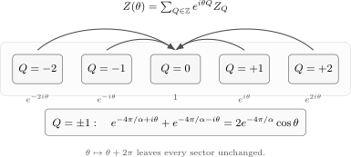
On closed oriented spacetime without an $SO(3)$ background twist, the path integral is a sum over integer topological sectors. Charge $Q$ carries the phase $e^{i\theta Q}$; the sum is $2\pi$ periodic, and the first instanton pair contributes through $2e^{-4\pi/\alpha}\cos\theta$. This is a schematic sector decomposition, not a transition among sectors through the arrows.

The theta term is locally a total derivative. It does not change the local instanton equations, and the same holomorphic maps are the classical saddles. Its effect is global: it changes the interference among disconnected sectors.

Charge reversal and the special angle theta = pi

For the symmetry discussion use closed spacetime, rather than selecting one fixed $\mathbf n_\infty$ at infinity. Define the internal transformation $\mathsf C:\mathbf n\mapsto-\mathbf n$. It preserves the kinetic term and reverses the target-sphere degree:

$$Q\mapsto -Q.$$

This is an internal unitary charge reversal, not an assumption about physical time reversal. In $CP^1$ variables $\mathbf n=z^\dagger\boldsymbol\sigma z$, it is $z\mapsto i\sigma^2z^*$; its square on $z$ is the gauge transformation $z\mapsto-z$. It maps the theory at $\theta$ to the theory at $-\theta$. Ordinary periodicity allows a symmetry at

$$\theta\equiv -\theta \pmod{2\pi}.$$

Thus the special charge-reversal-invariant angles are

$$\theta=0, \qquad \theta=\pi \pmod{2\pi}.$$

At $\theta=0$, all sectors have real positive theta phase. At $\theta=\pi$,

$$e^{i\pi Q}=(-1)^Q,$$

so every odd topological sector changes sign relative to $\theta=0$. This is not a small continuous perturbation. It is a different interference pattern protected by a discrete symmetry.

The sign flip alone does not solve the infrared theory. A sharper constraint follows by testing both $SO(3)$ and $\mathsf C$ with a background. On a closed oriented surface $\Sigma$, let $P$ be an $SO(3)$ background bundle and

$$b=\int_\Sigma w_2(P)\pmod 2\in\{0,1\}.$$

The second Stiefel–Whitney class $w_2$ measures whether $P$ lifts to an $SU(2)$ bundle. For $b=1$, its doublet transition functions close only up to a minus sign. The auxiliary $U(1)$ gauge phases in the $CP^1$ description compensate that sign; their flux, and hence the covariant topological charge, is half-integral. Thus

$$Q\in\mathbb Z+{b\over2},\qquad Z(\theta+2\pi;P)=(-1)^b Z(\theta;P).$$

The covariant charge in this formula includes the background connection; it is not the ordinary-derivative expression for $Q$ applied unchanged to a twisted field. At $\theta=\pi$, reversal changes each weight by

$$e^{-i\pi Q}=(-1)^b e^{i\pi Q}.$$

The possible two-dimensional topological counterterms for this $SO(3)$ background multiply $Z$ by $(-1)^{p b}$, $p=0,1$. They are $\mathsf C$ invariant and cannot remove the relative sign for $b=1$. This is the mixed $SO(3)$–$\mathsf C$ anomaly. The flux condition and counterterm obstruction are developed in Komargodski et al. 2018, preprint pp. 7–10, Eqs. (8)–(15), PDF. Their opposite Euclidean theta-sign choice reverses the theta label; this mod-two phase is unchanged. Composing their doublet conjugation with a flavor rotation gives our antipodal $\mathsf C$.

In a local unitary relativistic theory with these symmetries, the anomaly excludes a unique trivially gapped infrared state preserving both $SO(3)$ and $\mathsf C$. Gapless behavior or degenerate vacua breaking $\mathsf C$ can match it. It does not select a unique gapless theory. The separate roles of internal charge reversal and spacetime symmetries are explicit in Sulejmanpasic and Tanizaki 2018, pp. 2, 6–7, Eq. (29), PDF.

For the undeformed $O(3)$ model at $\theta=\pi$, the standard infrared identification is the gapless level-one $SU(2)$ Wess–Zumino–Witten theory. This uses dynamical information beyond the anomaly and the dilute gas; see Komargodski et al. 2018, § 2.4, preprint pp. 22–23, PDF. In particular, the cosine energy below does not establish that endpoint. For the uniform spin chain in the continuum regime of lesson 30,

$$\theta=2\pi S,$$

so integer spin corresponds to $\theta=0\pmod{2\pi}$ and half-integer spin corresponds to $\theta=\pi\pmod{2\pi}$. The distinction is discrete, not perturbatively small.

The one-instanton measure and the scale modulus

The following semiclassical profiles are defined on the Euclidean plane, separately from the general closed-surface background used to test the anomaly. Hold $\mathbf n_\infty$ fixed at Euclidean infinity. A convenient charge-one representative is then $w(z)=\rho e^{i\chi}/(z-X)$, with four real collective coordinates: a center $X\in\mathbb R^2$, a size $\rho>0$, and the residual target-space $U(1)$ angle $\chi$. In a large finite regulator, these are local plane approximations: sizes must be much smaller than each infrared length, and centers must lie far from any boundary compared with the size. A general closed surface need not admit this exact degree-one holomorphic saddle. If one instead integrates over the full global $O(3)$ orbit, additional orientation coordinates and the corresponding group volume must be treated consistently. With the fixed-boundary convention, the measure is schematically

$$Z_1(\theta) \sim \int d^2X\,{d\rho\over\rho^3}\,d\chi\, C(\alpha) \exp\left[-{4\pi\over\alpha}+i\theta\right],$$

where $C(\alpha)$ denotes determinant and zero-mode normalization factors. The precise prefactor is regulator-dependent; the important pieces are the collective-coordinate measure, the exponential $e^{-4\pi/\alpha}$, and the phase $e^{i\theta}$. The measure shown here is not the measure over all six real parameters of a general Möbius transformation: fixing the boundary value removes the two global target orientations that would move $\mathbf n_\infty$.

Classically the instanton has no preferred size. Quantum mechanically, an instanton of size $\rho$ probes momenta of order

$$\mu\sim {1\over\rho}.$$

The classical exponential should therefore be RG-improved by using the running coupling $\alpha(1/\rho)$. Let $\alpha_0=\alpha(\Lambda_{\rm UV})$ at a weakly coupled ultraviolet reference scale. The one-loop $O(3)$ running gives

$${1\over\alpha(\mu)}={1\over\alpha_0}+{1\over2\pi}\log {\mu\over\Lambda_{\rm UV}}.$$

Setting $\mu=1/\rho$,

$${1\over\alpha(1/\rho)} ={1\over\alpha_0}-{1\over2\pi}\log(\rho\Lambda_{\rm UV}),$$

and hence

$$\exp\left[-{4\pi\over\alpha(1/\rho)}\right] = \exp\left[-{4\pi\over\alpha_0}\right](\rho\Lambda_{\rm UV})^2.$$

Thus the running coupling turns the naive size dependence into

$${d\rho\over\rho^3} \exp\left[-{4\pi\over\alpha(1/\rho)}\right] \sim \Lambda_{\rm UV}^2e^{-4\pi/\alpha_0}{d\rho\over\rho}.$$

Define the one-loop RG scale

$$\Lambda_\sigma=\mu e^{-2\pi/\alpha(\mu)} =\Lambda_{\rm UV}e^{-2\pi/\alpha_0}.$$

It is independent of the reference scale at this order, and the preceding prefactor is $\Lambda_\sigma^2$. It is not a definition of the physical mass gap, which depends on theta and can vanish at $\theta=\pi$. The extrapolation $\rho\sim\Lambda_\sigma^{-1}$ marks loss of weak-coupling control, not a derived sharp cutoff.

There is a distinct ultraviolet issue even if the upper end remains weakly coupled. Keep an explicit minimum size $a$ and maximum size $R$ with $a<R\ll\Lambda_\sigma^{-1}$ and small $\alpha(1/R)$. For the finite rectangular regulator used below, also require $R\ll\min(L,\beta)$, where $L$ is the spatial length and $\beta$ the Euclidean time extent; omitted boundary or image corrections must be controlled separately. With a constant schematic determinant factor $C_0$ (including the angle integral), the fugacity per Euclidean area is

$$\zeta(a,R)\simeq C_0\Lambda_\sigma^2\int_a^R{d\rho\over\rho} =C_0\Lambda_\sigma^2\log{R\over a}.$$

Here $[\zeta]=\text{mass}^2$. Shrinking $a$ by a decade adds $C_0\Lambda_\sigma^2\log 10$ in this schematic approximation. Determinants and higher running can add coupling powers and logarithms; setting them constant is not an exact density calculation. The small-instanton problem is nevertheless real and cannot be repaired by an infrared cutoff. The $CP^1=O(3)$ size dependence and the distinction between continuum small instantons and lattice dislocations are discussed in Bonanno, D’Elia and Margari 2023, preprint p. 2, Eqs. (5)–(6), and p. 4, Eqs. (16)–(17), PDF.

The diagram separates this finite weak band from the strong region. Inspect the lower endpoint as well as the decreasing inverse coupling.

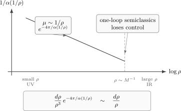
Schematic one-loop running with $a<\rho<R\ll\Lambda_\sigma^{-1}$. The size weight is $\Lambda_\sigma^2d\rho/\rho$ before determinant factors. Every extra small-size decade contributes again; the dashed continuation toward $\Lambda_\sigma^{-1}$ only estimates where weak coupling fails. The horizontal coordinate is dimensionless, and $\Lambda_\sigma$ is an RG scale rather than a theta-independent physical mass gap.

Thus a finite regulated size calculation can reveal topology and theta dependence without settling either the removal of its ultraviolet prescription or the full infrared dynamics.

Dilute gas and vacuum energy

If instantons and anti-instantons are dilute and approximately independent, their sum becomes a grand canonical gas. Mixed instanton–anti-instanton configurations are not exact holomorphic multi-instanton saddles; here they are approximate, widely separated constituents whose interactions are neglected at leading order. Keep the cutoffs fixed and write $\zeta=\zeta(a,R)>0$ for the single-constituent fugacity, including determinant and angle factors but excluding the center integral $V$. Let $Z_{\rm pert}$ denote the zero-constituent background; it differs from the full sector $Z_{Q=0}$, which also contains neutral pairs. A configuration with $N_+$ instantons and $N_-$ anti-instantons has charge

$$Q=N_+-N_-,$$

and contributes

$${(V\zeta)^{N_+}\over N_+!} {(V\zeta)^{N_-}\over N_-!} e^{i\theta(N_+-N_-)}.$$

Summing over $N_+$ and $N_-$ gives

$${Z(\theta)\over Z_{\rm pert}} \approx \sum_{N_+,N_-\ge0} {(V\zeta e^{i\theta})^{N_+}\over N_+!} {(V\zeta e^{-i\theta})^{N_-}\over N_-!} = \exp\left[2V\zeta\cos\theta\right].$$

Write the Euclidean area as $V=\beta L$, keeping the time extent and spatial length distinct. For a thermal trace, $\beta$ is the inverse temperature. At fixed size cutoffs, write $f_V$ as shorthand for the finite-regulator free-energy density; its geometry is specified by $(\beta,L)$, not by their product alone. The vacuum energy density requires the zero-temperature limit first and then the spatial thermodynamic limit, assuming these limits exist:

$$\begin{aligned} f_V(\theta)&=-{1\over\beta L}\log Z_{\beta,L}(\theta),\\ f(\theta)&=\lim_{L\to\infty}\lim_{\beta\to\infty}f_V(\theta). \end{aligned}$$

Taking $L\to\infty$ at fixed $\beta$ instead gives a thermal free-energy density. The ideal independent gas above neglects finite-geometry effects and takes $\zeta(a,R)$ to be independent of $\beta$ and $L$; its theta-dependent density is therefore the same before and after the displayed limits. Subtracting the value at $\theta=0$ gives

$$f(\theta)-f(0)=2\zeta(1-\cos\theta).$$

The regulated gas susceptibility is therefore

$$\chi_t={\partial^2 f\over\partial\theta^2}\bigg|_{\theta=0}=2\zeta.$$

Dividing by $2\zeta$ displays the predicted shape without hiding the cutoff dependence in the vertical scale.

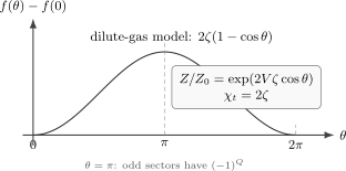
The graph is the quantitative shape $[f(\theta)-f(0)]/(2\zeta)=1-\cos\theta$ of the independent gas at fixed $\zeta(a,R)>0$. Its dimensional susceptibility is $\chi_t=2\zeta(a,R)$; neither a finite continuum susceptibility nor the true $O(3)$ endpoint at $\theta=\pi$ follows from this model.

The exact regulated function $f(\theta)$ can be more complicated, especially near $\theta=\pi$. Untwisted periodicity, charge-reversal symmetry and the paired theta phases survive beyond the independent-gas assumption.

The finite-volume derivative identities follow directly by differentiating the regulated sector sum, independently of a dilute approximation:

$$\begin{aligned} {\partial f_V\over\partial\theta}&=-{i\over V}\langle Q\rangle_\theta,\\ \left.{\partial^2 f_V\over\partial\theta^2}\right|_0 &={\langle Q^2\rangle_0-\langle Q\rangle_0^2\over V}\ge0. \end{aligned}$$

The inequality uses the positive theta-zero measure. In the gas, independent Poisson variables have $\operatorname{Var}Q=\operatorname{Var}N_++\operatorname{Var}N_-=2V\zeta$, reproducing $\chi_t=2\zeta$. These are identities at a specified regulator. Taking a thermodynamic limit, interchanging limits and derivatives, and removing the ultraviolet prescription are separate questions. In particular, they do not establish finite continuum $O(3)$ susceptibility.

Instanton corrections to running couplings

Perturbation theory in the $Q=0$ sector gives a beta function independent of $\theta$:

$$\beta_{\rm pert}(\alpha) =-{\alpha^2\over2\pi}+O(\alpha^3).$$

Instantons can add nonanalytic corrections. Since the charge-$\pm1$ sectors carry phases $e^{\pm i\theta}$, a charge-reversal-even Wilsonian flow equation can contain terms of the schematic form

$$\delta\beta(\alpha,\theta) \propto e^{-4\pi/\alpha}(e^{i\theta}+e^{-i\theta}) =2e^{-4\pi/\alpha}\cos\theta.$$

Thus one may write schematically

$$\beta(\alpha,\theta) =-{\alpha^2\over2\pi}+O(\alpha^3) -C(\alpha)e^{-4\pi/\alpha}\cos\theta +O(e^{-8\pi/\alpha}),$$

where $C(\alpha)$ depends on the running-coupling definition; its value or sign has not been calculated here. This is the allowed exponential and theta structure, not a determination of a universal nonperturbative beta function. The action and the beta coefficient must use the same coupling: if $u=\alpha/(2\pi)$, then $\beta_u=-u^2+\cdots$ but $S_{\rm inst}=2/u$, so the exponential is $e^{-2/u}$.

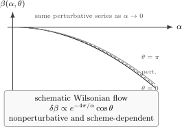
Perturbative running is blind to $\theta$. The first instanton correction carries the factor $e^{-4\pi/\alpha}\cos\theta$, so its sign flips between $\theta=0$ and $\theta=\pi$. The drawing is schematic; the prefactor depends on the definition of the running coupling.

At very weak coupling this correction is incredibly small. But the RG flow drives the theory toward larger $\alpha$ in the infrared. Once the flow reaches strong coupling, the distinction between $\theta=0$ and $\theta=\pi$ is no longer parametrically tiny.

This is the main reader-facing lesson of the page. Perturbation theory says that all theta angles look identical near the ultraviolet fixed point. Instantons explain how the theta angle re-enters through effects that are invisible order by order in $\alpha$. Strong infrared dynamics can then amplify those initially tiny differences.

Plasma language and the mass gap

The holomorphic multi-instantons of the $O(3)$ model can be written as rational maps,

$$w(z)=C\prod_{j=1}^k{z-a_j\over z-b_j}.$$

The points $a_j$ and $b_j$ are zeros and poles of the stereographic coordinate $w$. They are collective coordinates of a degree-$k$ map, not literal instantons and anti-instantons. Nevertheless, the collective-coordinate measure contains logarithmic interactions among these moduli, so it resembles a two-dimensional Coulomb plasma.

In an ordinary two-dimensional Coulomb plasma, screening replaces scale-free correlations by a finite screening length. The rational-map measure suggests the analogous mechanism here. In field-theory language, such a finite correlation length would be a mass gap:

$$\xi<\infty, \qquad M\sim \xi^{-1}>0.$$

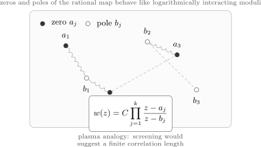
The rational-map moduli of multi-instantons resemble a logarithmically interacting two-dimensional plasma. This is an auxiliary collective-coordinate picture: zeros and poles are moduli of $w(z)$, not separate topological charges. The screening analogy suggests, but does not by itself derive, a finite correlation length.

Here $M$ denotes a physical inverse correlation length if one is generated; it must not replace the running scale $\Lambda_\sigma$ at every theta. The analogy prepares the next lesson: under its weak-coupling and heavy-core assumptions, compact three-dimensional gauge theory has a monopole Coulomb gas whose screening produces a mass and an area law. The sigma-model moduli picture alone does not establish that conclusion.

Summary

The theta angle weights integer topological sectors by

$$e^{i\theta Q}.$$

On closed untwisted spacetime the theory is $2\pi$ periodic, and $\mathsf C:\mathbf n\mapsto-\mathbf n$ maps $\theta$ to $-\theta$. The invariant angles are $\theta=0$ and $\theta=\pi$. At $\theta=\pi$, the mixed $SO(3)$–$\mathsf C$ anomaly excludes a unique trivially gapped state preserving both symmetries; it does not by itself derive the $SU(2)_1$ infrared identification.

Instantons generate nonperturbative factors

$$e^{-4\pi/\alpha+i\theta},$$

while anti-instantons generate

$$e^{-4\pi/\alpha-i\theta}.$$

For charge-reversal-even observables the leading paired theta factor is therefore

$$2e^{-4\pi/\alpha}\cos\theta.$$

The one-instanton size modulus links semiclassics to RG flow. Running-coupling improvement changes the naive size measure into a logarithmic integral,

$${d\rho\over\rho^3}e^{-4\pi/\alpha(1/\rho)} \sim {d\rho\over\rho},$$

up to overall scale and determinant factors. A finite weak band $a<\rho<R$ gives $\log(R/a)$ at this schematic order, so the ultraviolet endpoint needs its own prescription. The separate scale $\rho\sim\Lambda_\sigma^{-1}$ marks where the one-loop density loses control; it is not a theta-independent physical correlation length.

A dilute gas at fixed cutoffs, with $\zeta=\zeta(a,R)$, gives

$$f(\theta)-f(0)=2\zeta(1-\cos\theta), \qquad \chi_t=2\zeta.$$

More generally, instantons can correct Wilsonian flow equations by terms such as

$$\delta\beta\sim e^{-4\pi/\alpha}\cos\theta.$$

The sign flip at $\theta=\pi$ helps distinguish the sectors, while their actual infrared dynamics and the continuum susceptibility require more information.

Common pitfalls

Discarding the theta term because it is locally a total derivative. Its integral labels disconnected sectors, and the relative phase between sectors affects the quantum theory.

Expecting perturbation theory to know about $\theta$. Perturbation theory around a trivial vacuum lives in $Q=0$, so its beta function is theta independent.

Treating the $O(3)$ instanton gas as uniformly controlled. Small instantons accumulate toward the ultraviolet, even if the upper size stays weakly coupled. At the other end, $\Lambda_\sigma^{-1}$ estimates loss of control; it neither supplies a derived sharp cutoff nor fixes the physical mass at every theta.

Inferring a continuum susceptibility from $\chi_t=2\zeta$. This identity describes a specified independent gas. Removing the regulator can change or destroy the limit, and the exact finite-volume charge-variance identity does not resolve that question.

Assigning a universal coefficient to $e^{-4\pi/\alpha}\cos\theta$ in a beta function. The coefficient depends on the definition of the running coupling. The theta structure and exponential order are the robust facts.

Calling zeros and poles separate instantons and anti-instantons. They are moduli of one holomorphic multi-instanton map, although their measure has a useful plasma-like interpretation.

Exercises

Exercise 1: Periodicity from integer charge

Show that the theta-dependent partition function is $2\pi$ periodic if $Q\in\mathbb Z$.

Solution

Using

$$Z(\theta)=\sum_{Q\in\mathbb Z}e^{i\theta Q}Z_Q,$$

we find

$$Z(\theta+2\pi) =\sum_{Q\in\mathbb Z}e^{i\theta Q}e^{i2\pi Q}Z_Q.$$

Since $Q$ is an integer, $e^{i2\pi Q}=1$. Hence

$$Z(\theta+2\pi)=Z(\theta).$$

Exercise 2: Charge reversal and the background test

Use $\mathsf C:Q\mapsto-Q$ to find the invariant theta angles in the untwisted theory. Then take an $SO(3)$ background with $b=1$ and $Q\in\mathbb Z+1/2$: show why multiplying the partition function by either allowed counterterm $(-1)^{p b}$ fails to restore simultaneous background gauge invariance and $\mathsf C$ at $\theta=\pi$. Does the obstruction identify a unique infrared conformal theory?

Solution

The theta factor transforms as

$$e^{i\theta Q}\mapsto e^{-i\theta Q}=e^{i(-\theta)Q}.$$

Thus $\mathsf C$ maps the theory at $\theta$ to the theory at $-\theta$. In the untwisted problem it can be a symmetry only if

$$-\theta\equiv\theta\pmod{2\pi}.$$

This gives

$$2\theta=2\pi k, \qquad k\in\mathbb Z,$$

so

$$\theta=0,\pi\pmod{2\pi}.$$

The integer sectors still have different weights: phase one at zero theta and $(-1)^Q$ at pi. In the background $b=1$, every allowed $Q$ is half-integral, so

$$\frac{e^{-i\pi Q}}{e^{i\pi Q}}=e^{-2\pi iQ}=-1.$$

The factor $(-1)^{p b}$ is unchanged under $\mathsf C$ and multiplies both weights equally, leaving their relative minus sign. This tests the anomalous transformation of the weights; it does not divide by a possibly vanishing partition function. A unique trivially gapped symmetric infrared state cannot reproduce this response. Gaplessness or symmetry breaking can; choosing the particular $SU(2)_1$ endpoint requires the additional dynamics discussed above.

Exercise 3: RG improvement of the size integral

Using

$${1\over\alpha(\mu)}={1\over\alpha_0}+{1\over2\pi}\log {\mu\over\Lambda_{\rm UV}},$$

show that

$${d\rho\over\rho^3} \exp\left[-{4\pi\over\alpha(1/\rho)}\right]$$

is proportional to $d\rho/\rho$ up to a $\rho$-independent factor. Neglect the running of the determinant factor, integrate over $a<\rho<R\ll\Lambda_\sigma^{-1}$, and compute the change when $a$ is replaced by $a/10$. Explain separately what fails near $\rho\sim\Lambda_\sigma^{-1}$.

Solution

Set $\mu=1/\rho$:

$${1\over\alpha(1/\rho)} ={1\over\alpha_0}+{1\over2\pi}\log {1\over\rho\Lambda_{\rm UV}} ={1\over\alpha_0}-{1\over2\pi}\log(\rho\Lambda_{\rm UV}).$$

Therefore

$$-{4\pi\over\alpha(1/\rho)} =-{4\pi\over\alpha_0}+2\log(\rho\Lambda_{\rm UV}),$$

so

$$\exp\left[-{4\pi\over\alpha(1/\rho)}\right] =e^{-4\pi/\alpha_0}(\rho\Lambda_{\rm UV})^2.$$

Multiplying by $d\rho/\rho^3$ gives

$${d\rho\over\rho^3} \exp\left[-{4\pi\over\alpha(1/\rho)}\right] = \Lambda_{\rm UV}^2e^{-4\pi/\alpha_0}{d\rho\over\rho}.$$

The prefactor is $\Lambda_\sigma^2$, independent of $\rho$. The finite integral is

$$\Lambda_\sigma^2\log(R/a),\qquad \Delta=\Lambda_\sigma^2\log 10.$$

Multiply both by the chosen constant determinant/angle factor to obtain the schematic fugacity. Adding an ultraviolet decade gives a nonzero increment although the upper size remains weakly coupled. By contrast, near $\rho\sim\Lambda_\sigma^{-1}$ the one-loop extrapolation of $\alpha(1/\rho)$ is no longer small. This is a breakdown estimate, not a derived step-function cutoff or an identification of the physical theta-dependent mass.

Exercise 4: Dilute-gas exponentiation

For the independent gas at fixed cutoffs and $\zeta=\zeta(a,R)>0$, derive

$${Z(\theta)\over Z_{\rm pert}}=\exp(2V\zeta\cos\theta)$$

and compute $\chi_t$ both by differentiation and by charge variance. Why is $Z_{\rm pert}$ different from the complete $Q=0$ sector, and what does this calculation leave undecided about a continuum limit?

Solution

A configuration with $N_+$ instantons and $N_-$ anti-instantons has topological charge

$$Q=N_+-N_-.$$

The dilute-gas sum is

$${Z(\theta)\over Z_{\rm pert}} = \sum_{N_+,N_-\ge0} {(V\zeta e^{i\theta})^{N_+}\over N_+!} {(V\zeta e^{-i\theta})^{N_-}\over N_-!}.$$

The two sums exponentiate independently:

$${Z(\theta)\over Z_{\rm pert}} =e^{V\zeta e^{i\theta}}e^{V\zeta e^{-i\theta}} =e^{2V\zeta\cos\theta}.$$

Thus

$$f(\theta)-f(0)=2\zeta(1-\cos\theta),$$

and

$$\chi_t={\partial^2 f\over\partial\theta^2}\bigg|_{\theta=0}=2\zeta.$$

At theta zero, $N_\pm$ are independent Poisson variables of mean $V\zeta$, so $\langle Q\rangle=0$ and $\operatorname{Var}Q=2V\zeta$. Dividing by $V$ gives the same susceptibility. The full neutral sector includes all $N_+=N_-=n$:

$${Z_{Q=0}\over Z_{\rm pert}} =\sum_{n=0}^{\infty}{(V\zeta)^{2n}\over(n!)^2},$$

not just the $n=0$ background. The gas result does not remove the size prescription or control the large-instanton region, so it does not establish a finite continuum susceptibility.

References

• C. Bonanno, M. D’Elia and F. Margari, “Topological Susceptibility of 2d $CP^1$ or $O(3)$ Non-Linear Sigma-Model: Is It Divergent or Not?”, Physical Review D 107 (2023), 014515, doi:10.1103/PhysRevD.107.014515. Open PDF, arXiv:2208.00185v2.
• Z. Komargodski, A. Sharon, R. Thorngren and X. Zhou, “Comments on Abelian Higgs Models and Persistent Order,” SciPost Physics 6 (2019), 003, doi:10.21468/SciPostPhys.6.1.003. Open PDF, arXiv:1705.04786v4 (2018); locators above refer to this preprint.
• T. Sulejmanpasic and Y. Tanizaki, “C-P-T Anomaly Matching in Bosonic Quantum Field Theory and Spin Chains,” Physical Review B 97 (2018), 144201, doi:10.1103/PhysRevB.97.144201. Open PDF, arXiv:1802.02153v2.

Further reading

• I. Affleck, “Exact Critical Exponents for Quantum Spin Chains, Non-Linear Sigma Models at $\theta=\pi$ and the Quantum Hall Effect,” Nuclear Physics B 265 (1986), 409–447, doi:10.1016/0550-3213(86)90167-7.
• A. A. Belavin and A. M. Polyakov, “Metastable States of Two-Dimensional Isotropic Ferromagnets,” JETP Letters 22 (1975), 245.
• S. Coleman, Aspects of Symmetry: Selected Erice Lectures, Cambridge University Press, Cambridge, 1985, especially “The Uses of Instantons.”
• F. D. M. Haldane, “Continuum Dynamics of the 1-D Heisenberg Antiferromagnet: Identification with the $O(3)$ Nonlinear Sigma Model,” Physics Letters A 93 (1983), 464–468, doi:10.1016/0375-9601(83)90631-X.
• F. D. M. Haldane, “Nonlinear Field Theory of Large-Spin Heisenberg Antiferromagnets: Semiclassically Quantized Solitons of the One-Dimensional Easy-Axis Néel State,” Physical Review Letters 50 (1983), 1153–1156, doi:10.1103/PhysRevLett.50.1153.
• A. M. Polyakov, Gauge Fields and Strings, Contemporary Concepts in Physics, vol. 3, Harwood Academic Publishers, Chur, 1987.
• J. Zinn-Justin, Quantum Field Theory and Critical Phenomena, 5th ed., Oxford University Press, Oxford, 2021.