Primary Fields, Cylinder Maps, and Mode Expansions

The exponential map turns evolution on a Euclidean cylinder into radial evolution on the plane. This lesson uses that map to calculate a two-point function and the cylinder energy shift, then distinguishes two operations that are easy to confuse: a mode commutator acting on a displaced field and a local mode defining a descendant. We use ordinary primary fields with definite weights, a flat cylinder of circumference $2\pi$, and a specified state and spin or monodromy sector.

Required background. Stress-tensor OPE and conformal Ward identities supplies the primary OPE, positive contour action, and finite stress transformation. The discussion below uses those results with their stated contact and vacuum assumptions.

The exponential map and primary fields

Write the dimensionless cylinder coordinate as $w=\tau+i\varphi$, where $\varphi\sim\varphi+2\pi$ and $\tau\in\mathbb R$. The map

$$z=e^w=e^\tau e^{i\varphi}$$

identifies the cylinder with the punctured plane. Increasing $\tau$ increases the radius; increasing $\varphi$ moves counterclockwise. The origin and infinity correspond to infinite past and future cylinder time. Neither is the image of a finite cylinder point.

The metrics obey

$$ds_{\rm plane}^2=dz\,d\bar z =e^{2\tau}(d\tau^2+d\varphi^2).$$

Thus the map is conformal, not an isometry. Transport to a flat cylinder includes a Weyl rescaling and a compatible frame choice for fields with spin. For a primary of weights $(h,\bar h)$,

$$O_{\rm cyl}(w,\bar w) =z^h\bar z^{\bar h}O_{\rm plane}(z,\bar z), \qquad \Delta=h+\bar h,\quad s=h-\bar h.$$

The powers use consistent local branches. Their continuation around the spatial circle must also agree with the chosen sector; a local transformation law does not select that sector by itself. The finite primary law is discussed in Di Francesco, Mathieu and Sénéchal 1997, § 5.1.4, p. 116, Eqs. 5.21–5.23.

In the figure, compare the two marked cylinder slices with the two radii: a time translation by $\log 2$ doubles the radius. The angular direction and the identification of the strip edges are equally important.

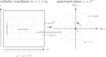
Equal-time cylinder circles become equal-radius plane circles under $z=e^{\tau+i\varphi}$. The marked slices have $\tau=0,\log 2$ and radii $1,2$. The origin and infinity are omitted ends of the cylinder map; local insertion data specify a state at an end. The drawing illustrates the conformal relation and does not identify the two flat metrics as equal.

A periodic spatial coordinate with noncompact Euclidean time describes a state evolving on a circle. It is not by itself a finite-temperature trace. The geometric and radial interpretation is developed in Di Francesco, Mathieu and Sénéchal 1997, § 6.1.1, pp. 151–153, Eqs. 6.1–6.12.

A two-point function on the cylinder

Take two separated primaries with a nonzero pairing in the plane vacuum, normalized to

$$G_{\rm plane} =\frac1{z_{12}^{2h}\bar z_{12}^{2\bar h}}, \qquad z_{12}=z_1-z_2.$$

The second field can be the conjugate of the first; its label is suppressed. Map this state and its insertions to the cylinder with compatible branches. Since

$$z_1-z_2 =2e^{(w_1+w_2)/2}\sinh\frac{w_{12}}2,$$

the primary factors cancel the dependence on the sum of the coordinates. The result is

$$G_{\rm cyl}(w_{12},\bar w_{12}) =\frac1{ \left(2\sinh\frac{w_{12}}2\right)^{2h} \left(2\sinh\frac{\bar w_{12}}2\right)^{2\bar h}}.$$

Exercise 2 gives the full cancellation. For spinning or chiral fields this expression retains its ordering and branch data; it need not be a positive real function.

For a spinless pairing with real dimension, $h=\bar h=\Delta/2$, the separated Euclidean kernel has a particularly useful real form:

$$\begin{aligned} G_{\rm cyl}(\tau,\varphi) &=[2(\cosh\tau-\cos\varphi)]^{-\Delta},\\ G_{\rm cyl}(0,\varphi) &=\left|2\sin\frac{\varphi}{2}\right|^{-2\Delta}. \end{aligned}$$

The absolute value surrounds the entire sine. Putting an absolute value only on its argument would not give a periodic expression for general noninteger $\Delta$.

Three checks explain the result. First, for small separation, $2(\cosh\tau-\cos\varphi)=\tau^2+\varphi^2+O(\tau^4+\varphi^4)$, recovering the plane power law. Second, the angular dependence is $2\pi$ periodic and singular only at coincident points modulo that period. Third, for $\tau>0$ at $\varphi=0$,

$$G_{\rm cyl}(\tau,0) =e^{-\Delta\tau}(1-e^{-\tau})^{-2\Delta}.$$

For $\Delta>0$, its convergent expansion is

$$G_{\rm cyl}(\tau,0) =\sum_{N=0}^{\infty} \frac{(2\Delta)_N}{N!}\, e^{-(\Delta+N)\tau}.$$

Here $(a)_0=1$ and $(a)_N=a(a+1)\cdots(a+N-1)$. The leading energy difference is $\Delta$, followed by integer descendant levels. These coefficients are aggregate two-point spectral weights, not counts of independent states. At $\Delta=0$ this normalized two-point function becomes constant, $G=1$; zero weights alone do not identify the field with the identity. The radial interpretation of these energy differences is the next step.

Radial states and the cylinder energy

Radial quantization uses circles around zero as equal-time slices. An insertion at the origin prepares a state on a surrounding circle,

$$|O\rangle=O(0)|0\rangle.$$

The notation denotes the state prepared by the disk path integral, or the corresponding radial representation construction. It is not an assertion that an unsmeared field is an everywhere-defined bounded operator. Reflection positivity gives the usual positive Hilbert-space interpretation in a unitary theory. Without it one must keep the radial representation and its pairing distinct from a positive Hilbert space.

The insertion can also specify a spin structure, twist or defect sector on the surrounding circle. In noncompact theories, some insertions prepare distributional or delta-normalizable states; normalizability requires a separate check. The two slices in the geometric figure describe the evolution of the same prepared state, with these boundary data held fixed.

For a primary state,

$$L_0|O\rangle=h|O\rangle,\qquad \bar L_0|O\rangle=\bar h|O\rangle.$$

The plane dilation and rotation generators are therefore $D=L_0+\bar L_0$ and $J=L_0-\bar L_0$. Cylinder energies have an additional constant, which can be calculated directly from the finite stress law of the previous lesson:

$$T_{\rm cyl}(w) =(f')^2T_{\rm plane}(f(w))+\frac c{12}\{f,w\}.$$

For $f=e^w$, all three derivatives equal $e^w$, so

$$\{e^w,w\}=1-\frac32=-\frac12, \qquad T_{\rm cyl}(w)=z^2T_{\rm plane}(z)-\frac c{24}.$$

The antiholomorphic stress has the corresponding shift $-\bar c/24$. The spatial averages of $T_{\rm cyl}+\bar T_{\rm cyl}$ and $T_{\rm cyl}-\bar T_{\rm cyl}$ give

$$\begin{aligned} H_{\rm cyl}&=L_0+\bar L_0-\frac{c+\bar c}{24},\\ P_{\rm cyl}&=L_0-\bar L_0-\frac{c-\bar c}{24}. \end{aligned}$$

These formulas use the chosen flat cylinder and orientation. In an anomaly-free theory with $c=\bar c$, they reduce to $H_{\rm cyl}=D-c/12$ and $P_{\rm cyl}=J$. A theory with unequal chiral charges needs its own consistent global background definition; the local stress transformation is not a proof of anomaly-free coupling to arbitrary geometry. The exponential stress transformation and its vacuum shift are given in Di Francesco, Mathieu and Sénéchal 1997, § 5.4.2, pp. 138–139, Eqs. 5.137–5.139.

The plane identity vacuum has zero plane stress, hence cylinder energy $E_{\mathbf1}=-(c+\bar c)/24$. Another sector’s lowest state may have nonzero weights $h_0,\bar h_0$ and energy $h_0+\bar h_0-(c+\bar c)/24$. The constant stress shift alone does not identify the ground state of every sector. When the identity vacuum and the operator state belong to the stated radial construction, their energy difference is $\Delta$, consistent with the large-time two-point function above.

For a physical circumference $\ell$, introduce the dimensionful coordinate $W=\tau_{\rm phys}+ix$, with $x\sim x+\ell$, and use $z=e^{2\pi W/\ell}$. Energies and momenta then acquire the overall factor $2\pi/\ell$. The stress acquires its squared factor, as required by dimension.

Stress modes and radial commutators

On a circle centered at zero, define

$$L_n=\frac1{2\pi i}\oint_0 dz\,z^{n+1}T(z), \qquad T(z)=\sum_{n\in\mathbb Z}L_nz^{-n-2}.$$

These are modes centered at the origin. Only $n=-1,0,1$ correspond to holomorphic vector fields regular on the whole sphere; arbitrary Laurent modes are not all global conformal transformations.

The primary OPE from the previous lesson is

$$T(z)O(a,\bar a)\sim \frac{h\,O(a,\bar a)}{(z-a)^2} +\frac{\partial_aO(a,\bar a)}{z-a}.$$

To compute a commutator at $a\ne0$, take the difference of radially outer and inner contours: both surround zero, and only the outer one surrounds $a$. Assume the intervening annulus has no other insertions, poles or cuts. Their difference can be deformed onto a small counterclockwise circle $C_a$ around $a$ that excludes zero. This gives

$$\begin{aligned} [L_n,O(a,\bar a)] &=\frac1{2\pi i}\oint_{C_a}dz\, z^{n+1}T(z)O(a,\bar a)\\ &=\left[a^{n+1}\partial_a+(n+1)h\,a^n\right]O(a,\bar a). \end{aligned}$$

The contour difference implements the two radial orderings; a single contour has not been moved through the origin. For $n\le-2$, the factor $z^{n+1}$ has a pole there. Keeping zero outside the swept annulus is essential. The nested-contour argument is developed in Di Francesco, Mathieu and Sénéchal 1997, § 6.1.2, pp. 154–155, Eqs. 6.13–6.18.

At the origin the nonsingular generators give $[L_{-1},O(0)]=\partial O(0)$, $[L_0,O(0)]=hO(0)$ and $[L_n,O(0)]=0$ for $n>0$. Do not obtain an action of $L_{-2},L_{-3},\ldots$ there by substituting zero into the displaced formula. Local descendants have a separate definition.

Local modes and descendant fields

About an insertion at $a$, use the local coordinate $\xi=z-a$ and define

$$(L_n^{(a)}O)(a) =\frac1{2\pi i}\oint_{C_a}dz\, (z-a)^{n+1}T(z)O(a).$$

The superscript records the center of the local mode. Inside radially ordered correlators on a disk containing no other insertion, this is the coefficient in

$$T(z)O(a)= \sum_{n\in\mathbb Z} (z-a)^{-n-2}(L_n^{(a)}O)(a).$$

For a primary, positive local modes vanish. The singular terms and the first regular terms give the following dictionary.

Power of $z-a$	Local mode	Field coefficient
$-2$	$L_0^{(a)}$	$hO(a)$
$-1$	$L_{-1}^{(a)}$	$\partial O(a)$
$k\ge0$	$L_{-k-2}^{(a)}$	A local descendant, beginning with $(L_{-2}^{(a)}O)(a)$

The regular terms matter: they define local composites beyond the primary transformation law. Repeated negative modes generate a conformal family, but null relations can identify or remove some of these formal descendants. A list of formal mode products is not a proof that all its entries are independent physical states. See Di Francesco, Mathieu and Sénéchal 1997, § 6.6.1, pp. 177–178, Eqs. 6.147–6.155 for the local-contour definition and its state correspondence.

The figure compares the weighting functions as well as the contour centers. In the upper panel, subtracting radial orderings keeps $z^{n+1}$. In the lower panel, the definition of a local descendant uses $(z-a)^{n+1}$.

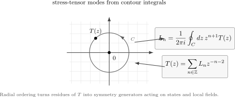
The difference of two counterclockwise radial contours isolates $a\ne0$ without crossing zero and retains the origin-mode weight $z^{n+1}$. A local descendant at $a$ uses $(z-a)^{n+1}$ instead. The radius $\rho$ of the local circle $C_a$ satisfies $0<\rho<|a|$, so it excludes zero. The swept annulus contains no other singularity or cut; for negative origin powers, its excluded central disk is essential. The diagram is schematic.

The identity field makes the distinction concrete:

$$(L_{-2}^{(a)}\mathbf1)(a)=T(a), \qquad [L_{-2},\mathbf1]=0.$$

Indeed, the first expression extracts the constant Taylor coefficient of $T(z)$ around $a$; the identity commutes with every global mode. The local descendant need not vanish even though the commutator does.

At the origin, the state–operator map identifies the state of $(L_n^{(0)}O)(0)$ with $L_n|O\rangle$. This does not imply that every local descendant is $[L_n,O(0)]$. Regularity of $T(z)|0\rangle$ at zero gives

$$L_n|0\rangle=0\quad(n\ge-1).$$

For $n\le-2$, the term $O(0)L_n|0\rangle$ cannot in general be discarded from a commutator acting on the vacuum. The vacuum and highest-weight conditions are stated in Di Francesco, Mathieu and Sénéchal 1997, § 6.2.2, pp. 157–158, Eqs. 6.26–6.37.

Chiral modes, spin and monodromy

Consider a chiral primary in a channel whose cylinder continuation is a scalar phase,

$$O_{\rm cyl}(w+2\pi i) =e^{-2\pi i\alpha}O_{\rm cyl}(w).$$

Its allowed mode numbers are $r\in\mathbb Z+\alpha$. The plane and cylinder expansions are

$$\begin{aligned} O_{\rm plane}(z) &=\sum_{r\in\mathbb Z+\alpha}O_rz^{-r-h},\\ O_{\rm cyl}(w) &=e^{hw}O_{\rm plane}(e^w) =\sum_{r\in\mathbb Z+\alpha}O_re^{-rw}. \end{aligned}$$

The power shift by $h$ ensures the ordinary cylinder Fourier dependence. The inverse formula is

$$O_r=\frac1{2\pi i}\oint_0dz\,z^{r+h-1}O_{\rm plane}(z).$$

The branch of the weighting factor compensates that of the field, so the integrand used for this mode extraction is single-valued in the specified channel. A field that mixes channels under continuation first requires that monodromy data; there need not be one common scalar shift for all matrix elements.

The spin or frame factor alone does not determine $\alpha$. If the plane field has monodromy $M$, then

$$O_{\rm plane}(e^{2\pi i}z)=M O_{\rm plane}(z), \qquad e^{-2\pi i\alpha}=e^{2\pi ih}M.$$

For a weight-$1/2$ Majorana field, a single-valued plane component has $M=1$, so the cylinder field is antiperiodic and its Neveu–Schwarz modes are half-integer. A Ramond insertion gives the plane branch $M=-1$, making the cylinder field periodic and its modes integer. These assignments, including their plane/cylinder distinction, are discussed in Di Francesco, Mathieu and Sénéchal 1997, §§ 6.4.1–6.4.2, pp. 169–170, Eqs. 6.101–6.109. We consistently use circumference $2\pi$; the period printed in Eq. 6.101 has an extra factor relative to the source’s surrounding circumference convention.

Substituting the plane mode expansion into the primary commutator provides another useful calculation. Differentiation gives

$$[L_n,O(z)] =\sum_r(nh-r)O_rz^{n-r-h}.$$

Setting $r=m+n$ and comparing the coefficient of $z^{-m-h}$ gives

$$[L_n,O_m]=[(h-1)n-m]O_{n+m}.$$

In particular, $[L_0,O_m]=-mO_m$: a negative mode raises the holomorphic weight by $-m$. This relation is an operator statement on the appropriate radial domains and channels; it does not declare that every mode acting on every state is nonzero.

Common pitfalls

Treating a conformal map as an isometry. The exponential map has a position-dependent Weyl factor. Primary Jacobians and the stress Schwarzian are part of transporting correlators between the two flat geometries.

Replacing a descendant by a commutator. Compare both the contour weight and the center. The identity example distinguishes them immediately.

Assuming the vacuum shift identifies every ground state. The stress shift is fixed by the central charges. A sector’s lowest weights and the existence of a normalizable vacuum are additional data.

Reading a spin factor as a complete boundary condition. Cylinder monodromy combines the frame factor with plane monodromy. Fix the channel before assigning integer or half-integer modes.

Exercises

Exercise 1: Quadratic-differential falloff at infinity

Let $T(z)dz^2$ be a quadratic differential. Show that if it is regular at $z=\infty$, then $T(z)=O(z^{-4})$ as $z\to\infty$. For the quantum stress tensor, apply this statement between the two Möbius inversion charts in the plane vacuum with no insertion at infinity.

Solution

Use the local coordinate near infinity

$$z'={1\over z}.$$

Then

$$dz'=-{dz\over z^2}, \qquad (dz')^2={dz^2\over z^4}.$$

A quadratic differential is coordinate independent:

$$T(z)dz^2=T'(z')(dz')^2.$$

Therefore

$$T(z)=T'(z'){1\over z^4}=T'(1/z){1\over z^4}.$$

If $T'(z')$ is regular at $z'=0$, then $T'(1/z)=T'(0)+O(1/z)$, and hence

$$T(z)=O(z^{-4}).$$

Exercise 2: Mapping a two-point function to the cylinder

Starting from the plane two-point function

$$\left\langle\mathcal O(z_1,\bar z_1)\mathcal O(z_2,\bar z_2)\right\rangle ={1\over z_{12}^{2h}\bar z_{12}^{2\bar h}},$$

derive the cylinder two-point function under $z=e^w$ on circumference $2\pi$. Use the mapped plane vacuum, a nonzero primary pairing, separated points and compatible branches in the specified sector.

Solution

The cylinder field is

$$\mathcal O_{\rm cyl}(w_i,\bar w_i) =z_i^h\bar z_i^{\bar h}\mathcal O_{\rm plane}(z_i,\bar z_i), \qquad z_i=e^{w_i}.$$

Thus

$$\left\langle\mathcal O_{\rm cyl}(w_1)\mathcal O_{\rm cyl}(w_2)\right\rangle = {(z_1z_2)^h(\bar z_1\bar z_2)^{\bar h}\over(z_1-z_2)^{2h}(\bar z_1-\bar z_2)^{2\bar h}}.$$

Now

$$z_1-z_2=e^{(w_1+w_2)/2}\left(e^{w_{12}/2}-e^{-w_{12}/2}\right) =2e^{(w_1+w_2)/2}\sinh{w_{12}\over2}.$$

The exponential prefactor cancels $(z_1z_2)^h=e^{h(w_1+w_2)}$, giving

$$\left\langle\mathcal O_{\rm cyl}(w_1,\bar w_1)\mathcal O_{\rm cyl}(w_2,\bar w_2)\right\rangle = {1\over\left(2\sinh{w_{12}\over2}\right)^{2h} \left(2\sinh{\bar w_{12}\over2}\right)^{2\bar h}}.$$

Exercise 3: Virasoro modes acting on a primary

Use the OPE

$$T(z)\mathcal O(a,\bar a) \sim {h\mathcal O(a,\bar a)\over(z-a)^2} +{\partial_a\mathcal O(a,\bar a)\over z-a}$$

to show that, for $a\ne0$ and a nested-contour annulus containing $a$ but no other singularity,

$$[L_n,\mathcal O(a,\bar a)] = \left(a^{n+1}\partial_a+(n+1)h a^n\right)\mathcal O(a,\bar a).$$

Then identify the local coefficients $(L_0^{(0)}\mathcal O)(0)$, $(L_{-1}^{(0)}\mathcal O)(0)$, and $(L_n^{(0)}\mathcal O)(0)$ for $n>0$.

Solution

By definition,

$$L_n={1\over2\pi i}\oint dz\,z^{n+1}T(z).$$

To compute the commutator, subtract the radially inner contour from the outer one. Both enclose zero, and only the outer one encloses $a$. Deform their difference onto a small circle around $a$ that excludes zero; no other singularity lies in the swept annulus. The residue is

$${1\over2\pi i}\oint_a dz\,z^{n+1} \left[ {h\mathcal O(a,\bar a)\over(z-a)^2} +{\partial_a\mathcal O(a,\bar a)\over z-a} \right].$$

The simple-pole term gives

$$a^{n+1}\partial_a\mathcal O(a,\bar a).$$

For the double pole, use

$${1\over2\pi i}\oint_a dz\,{f(z)\over(z-a)^2}=f'(a).$$

With $f(z)=z^{n+1}$, this gives

$$(n+1)a^n h\mathcal O(a,\bar a).$$

Therefore

$$[L_n,\mathcal O(a,\bar a)] = \left(a^{n+1}\partial_a+(n+1)h a^n\right)\mathcal O(a,\bar a).$$

At $a=0$, define the local coefficients through the OPE rather than taking a singular limit of the displaced negative-mode commutator:

$$T(z)\mathcal O(0) = \sum_m z^{-m-2}(L_m^{(0)}\mathcal O)(0).$$

Comparing with the primary OPE gives

$$(L_0^{(0)}\mathcal O)(0)=h\mathcal O(0), \qquad (L_{-1}^{(0)}\mathcal O)(0)=\partial\mathcal O(0), \qquad (L_n^{(0)}\mathcal O)(0)=0\quad(n>0).$$

References

• Di Francesco, Philippe, Pierre Mathieu, and David Sénéchal. Conformal Field Theory. Graduate Texts in Contemporary Physics. New York: Springer, 1997. DOI.

Further reading

The cylinder map and radial Hamiltonian develops the general-radius construction. The state–operator correspondence treats its assumptions and sector dependence in more detail.