Instantons in Quantum Mechanics and Vacuum Decay

Tunneling has no real classical trajectory through a forbidden region, yet it has a precise semiclassical description: after Wick rotation, the dominant path is a real saddle of the Euclidean action. In a degenerate double well that saddle is an instanton and splits energy levels; in a metastable potential it is a bounce and gives a decay rate. The same logic in field theory relates bounces, particle production, and the imaginary part of the in–out effective action.

This page develops that chain from one-dimensional WKB to false-vacuum decay. It also separates three quantities that are easy to conflate: a tunneling amplitude, a survival probability, and an inclusive production rate.

Required background. Euclidean continuation and Gaussian path integrals supplies the Wick rotation and saddle-point expansion used below.

Helpful background. WKB, eikonal approximation, and turning points reviews turning-point matching, while monopoles and confinement provides the field-theory instanton context from the preceding lesson.

Euclidean saddles and the inverted potential

The global convention is $\hbar=1$. To expose the semiclassical parameter temporarily, write

$$e^{iS}\quad\longrightarrow\quad e^{-S_E}, \qquad \text{or, with }\hbar\text{ restored,}\qquad e^{iS/\hbar}\quad\longrightarrow\quad e^{-S_E/\hbar}.$$

For one-dimensional quantum mechanics we write

$$S[x]=\int dt\,\left[{M\over2}\dot x^2-V(x)\right],$$

and under $t=-i\tau$,

$$S_E[x]=\int d\tau\,\left[{M\over2}(x')^2+V(x)\right], \qquad x'={dx\over d\tau}.$$

The Euclidean equation of motion is

$$Mx''=V'(x),$$

which is Newton’s equation in the inverted potential $-V(x)$. When discussing tunneling from a vacuum $x_0$, we often subtract the vacuum energy and use

$$U(x)=V(x)-V(x_0), \qquad U(x_0)=0.$$

Three semiclassical questions

It helps to separate three outputs. A degenerate double-well instanton gives a tunneling matrix element and an energy splitting. A false-vacuum bounce gives the imaginary part of a metastable energy and hence a decay rate. A background-field production saddle first gives the probability for the vacuum channel to survive; extracting a mean particle number or an exclusive multiplicity distribution may require additional information.

The real-time transition amplitude is formally

$$K(x_f,t_f;x_i,t_i) = \int_{x(t_i)=x_i}^{x(t_f)=x_f}\mathcal D x(t)\, \exp\left\{i\int_{t_i}^{t_f}dt\,\left[{M\over2}\dot x^2-V(x)\right]\right\}.$$

If a real classical trajectory connects the endpoints, the leading semiclassical contribution comes from stationary phase. The saddle obeys

$$M\ddot x=-V'(x).$$

Tunneling is different. In a classically forbidden region $V(x)>E$, the real-time momentum is imaginary, and no real classical path crosses the barrier. The useful saddle appears after the Wick rotation

$$t=-i\tau.$$

The action becomes

$$S_E[x]=\int d\tau\,\left[{M\over2}(x')^2+V(x)\right],$$

and stationarity gives

$$Mx''=V'(x).$$

The sign reversal is the whole story: Euclidean motion in $V$ is real-time motion in $-V$. A barrier of $V$ becomes a valley of $-V$, so a forbidden trajectory becomes an ordinary classical roll in imaginary time.

Because the Euclidean Lagrangian has no explicit $\tau$ dependence, there is a conserved quantity

$$\mathcal E_E={M\over2}(x')^2-V(x).$$

Indeed,

$${d\mathcal E_E\over d\tau} =x'\big(Mx''-V'(x)\big)=0.$$

If a finite-action trajectory approaches a minimum $x_0$ with $V(x_0)=0$ and $x'\to0$ at large $|\tau|$, then

$$\mathcal E_E=0.$$

Therefore along the tunneling trajectory,

$${M\over2}(x')^2=V(x), \qquad x'=\pm\sqrt{{2V(x)\over M}}.$$

This first-order equation is often the most efficient way to compute the semiclassical exponent.

WKB tunneling as Euclidean action

The connection with elementary WKB is direct. For a particle of energy $E$, define

$$p(x)=\sqrt{2M(E-V(x))}.$$

In the classically forbidden interval $x_1<x<x_2$, where $V(x)>E$, write

$$p(x)=i\kappa(x), \qquad \kappa(x)=\sqrt{2M(V(x)-E)}.$$

The WKB wavefunction decays through the barrier as

$$\psi(x)\sim \exp\left[-\int^x dx'\,\kappa(x')\right],$$

so the leading tunneling probability is

$$\boxed{ P_{\rm tunnel}(E)\sim \exp\left[-2\int_{x_1}^{x_2}dx\,\sqrt{2M(V(x)-E)}\right]. }$$

The factor of $2$ appears because probability is the squared magnitude of an amplitude. The same square root follows from Euclidean classical motion with shifted potential $V(x)-E$:

$${M\over2}(x')^2=V(x)-E.$$

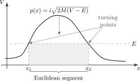
The forbidden interval $x_1<x<x_2$ contributes an imaginary real-time action, or equivalently a positive Euclidean action. The tunneling exponent is the integral of $\sqrt{2M(V-E)}$ between the turning points.

This is the first major nonperturbative pattern of the page. Perturbation theory produces powers of a coupling. Tunneling produces exponentials such as

$$e^{-\operatorname{const}/g}, \qquad e^{-\operatorname{const}/g^2}, \qquad e^{-\operatorname{const}/|E_{\rm ext}|},$$

depending on which parameter multiplies the action. Such terms have zero Taylor series around the weak-coupling point. They are not hidden at high loop order; they are outside ordinary perturbation theory.

Instantons in a degenerate double well

Now consider a symmetric double-well potential with two degenerate minima,

$$V(-a)=V(a)=0, \qquad V(x)>0\quad\text{for }-a<x<a.$$

A Euclidean instanton is a finite-action solution satisfying

$$x_I(\tau\to-\infty)=-a, \qquad x_I(\tau\to+\infty)=a, \qquad x_I'(\tau\to\pm\infty)=0.$$

The anti-instanton runs from $a$ to $-a$. Since the Euclidean energy vanishes, the instanton action is

$$S_0 = \int_{-\infty}^{\infty}d\tau\, \left[{M\over2}(x_I')^2+V(x_I)\right] = \int_{-\infty}^{\infty}d\tau\,2V(x_I).$$

Using $d\tau=dx/x'$ gives the useful formula

$$\boxed{ S_0=\int_{-a}^{a}dx\,\sqrt{2M V(x)}. }$$

Thus the instanton action is the one-way under-barrier WKB action.

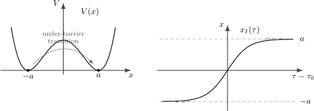
A double-well instanton connects two degenerate minima in imaginary time. In the inverted potential $-V(x)$, the instanton is an ordinary classical path rolling from one hilltop to the other.

For the quartic double well

$$V(x)={\lambda\over4}(x^2-a^2)^2, \qquad M=1,$$

the small-oscillation frequency at either minimum is

$$\omega^2=V''(a)=2\lambda a^2.$$

The first-order instanton equation is

$${dx\over d\tau}=\sqrt{\lambda\over2}(a^2-x^2),$$

for a path moving from $-a$ to $a$. Its solution is

$$\boxed{ x_I(\tau)=a\tanh{\omega(\tau-\tau_0)\over2}. }$$

The constant $\tau_0$ is the instanton center. It is a collective coordinate because translating the instanton in Euclidean time costs no action. The action is

$$S_0=\int_{-a}^{a}dx\,\sqrt{2V(x)} ={2\over3}a^2\omega.$$

A one-instanton contribution to the Euclidean transition amplitude has the schematic form

$$\langle a|e^{-HT}|-a\rangle_{1\text{-inst}} \sim K T e^{-S_0},$$

where $K$ is a fluctuation determinant with the translation zero mode removed. Summing a dilute gas of instantons and anti-instantons gives an energy splitting

$$\Delta E\sim 2K e^{-S_0}.$$

The exact prefactor depends on the determinant normalization. The exponential $e^{-S_0}$ is the robust semiclassical signature.

False vacua and bounces

An instanton between degenerate vacua mixes states; it does not make the vacuum disappear. Decay is described by a different saddle. In quantum mechanics, assume a metastable well with an escape channel and an outgoing-resonance prescription. A local minimum that is not the global minimum is insufficient: a closed confining double well has real discrete energies and coherent returns, not an exact irreversible decay rate. The complex resonance energy is defined by analytic continuation, not as an eigenvalue of the self-adjoint Hamiltonian Coleman 1985, ch. 7, § 2.4, pp. 279–282.

Let $x_f$ denote the metastable minimum and choose the escape direction as increasing $x$, so its outer turning point satisfies $x_t>x_f$. Subtract the false-well energy,

$$U(x)=V(x)-V(x_f), \qquad U(x_f)=0.$$

A bounce is a Euclidean solution satisfying

$$x_B(\tau\to\pm\infty)=x_f, \qquad x_B'(\tau\to\pm\infty)=0.$$

It leaves the false vacuum, reaches a turning point $x_t$ where

$$U(x_t)=0, \qquad x_B'(\tau_0)=0,$$

and returns. The Euclidean energy is again zero:

$${M\over2}(x_B')^2=U(x_B).$$

Because the path goes out and back, the bounce action is

$$\boxed{ B=2\int_{x_f}^{x_t}dx\,\sqrt{2M U(x)}. }$$

The leading decay rate has the form

$$\boxed{ \Gamma=Ae^{-B/\hbar}\big[1+O(\hbar)\big], }$$

where $A$ has dimensions of frequency and comes from fluctuations and the translation collective coordinate. We keep $\hbar$ visible in this formula to distinguish the classical bounce action $B$ from the dimensionless exponent; subsequent formulas again set $\hbar=1$.

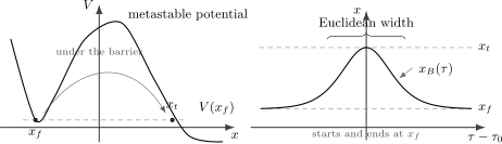
A false-vacuum bounce starts near the metastable minimum $x_f$, reaches the turning point $x_t$, and returns. The factor of two in $B=2\int dx\,\sqrt{2MU}$ comes from the outgoing and returning parts of the path.

The decay bounce is not a local minimum of the Euclidean action. The leading bounce has exactly one physical negative fluctuation mode. That fact is essential: the appropriate analytic continuation of that direction gives an imaginary contribution to the false-vacuum energy. A stationary configuration with more than one negative mode is not the leading decay saddle.

To see the connection, suppose an isolated narrow resonance dominates the false-well persistence amplitude in an exponential-decay time window, after the initial transient:

$$\langle F|e^{-iHT}|F\rangle \sim e^{-iE_fT}, \qquad E_f=E_R-{i\over2}\Gamma.$$

Then

$$|\langle F|e^{-iHT}|F\rangle|^2 \sim e^{-\Gamma T}.$$

Thus

$$\Gamma=-2\,\operatorname{Im}E_f.$$

The bounce calculation is a semiclassical way to compute this imaginary part with the decaying boundary prescription. This is not an exact arbitrarily late-time asymptotic formula: the real spectral measure also permits nonexponential tails, and a discrete closed system can recur. The field-theory rate below concerns nucleation in a large spatial volume and requires its own dilute-event limit.

The negative mode and the determinant

Expand around the bounce,

$$x(\tau)=x_B(\tau)+\eta(\tau).$$

To quadratic order,

$$S_E[x]=B+{1\over2}\int d\tau\,\eta(\tau)\mathcal M_B\eta(\tau)+\cdots,$$

where

$$\mathcal M_B=-M{d^2\over d\tau^2}+U''(x_B(\tau)).$$

There is a zero mode

$$\eta_0(\tau)\propto x_B'(\tau),$$

because the center of the bounce may be translated. There is also one negative eigenvalue. An ordinary real Gaussian integral along that direction would diverge. Defining the metastable state by analytic continuation and deforming to the relevant steepest-descent contour supplies an imaginary factor; the fact that only one side of the saddle contributes gives the conventional factor $i/2$ in the one-bounce term. The sign is fixed by requiring a decaying, rather than growing, state.

Schematic one-dimensional formulas look like

$$\Gamma = \left({B\over2\pi}\right)^{1/2} \left| {\det{}'\mathcal M_B\over\det\mathcal M_f} \right|^{-1/2} e^{-B} \times (\text{normalization factors}),$$

where $\det{}'$ means the zero mode is omitted and treated as a collective coordinate, while

$$\mathcal M_f=-M{d^2\over d\tau^2}+U''(x_f)$$

is the harmonic fluctuation operator in the false vacuum. The exponent is simple; the prefactor knows about the whole fluctuation spectrum.

In field theory, the bounce has one translation zero mode for each Euclidean coordinate. These zero modes are not ordinary Gaussian fluctuations; they are collective coordinates for the bubble center. Integrating them gives the Euclidean spacetime volume $T\mathcal V_{d-1}$. Dividing by that factor produces a decay rate per spatial volume. Schematically, in $d$ Euclidean spacetime dimensions,

$${\Gamma\over\mathcal V_{d-1}} \sim \left({B\over2\pi}\right)^{d/2} \left|{\det{}'\mathcal M_B\over\det\mathcal M_f}\right|^{-1/2} e^{-B},$$

up to renormalization and convention-dependent normalization factors. The prime again means that the zero modes are omitted from the determinant and treated as collective coordinates. The one negative mode is handled separately; it is what supplies the imaginary part.

Field-theory bounces

In field theory, the coordinate $x(\tau)$ is replaced by a field configuration. For a scalar field in $d$ Euclidean spacetime dimensions,

$$S_E[\phi]=\int d^dx\,\left[{1\over2}(\partial_\mu\phi)^2+V(\phi)\right].$$

If $\phi_f$ is the false vacuum, the bounce $\phi_B$ satisfies

$$-\partial^2\phi_B+V'(\phi_B)=0, \qquad \phi_B(x)\to\phi_f\quad\text{as }|x|\to\infty.$$

The exponent is

$$B=S_E[\phi_B]-S_E[\phi_f],$$

and the decay rate per spatial volume has the form

$${\Gamma\over\mathcal V_{d-1}}=A e^{-B}.$$

For one scalar with a canonical kinetic term in flat spacetime at zero temperature, the least-action bounce can be chosen $O(d)$ symmetric. This conclusion is not automatic for thermal decay, gravity, noncanonical kinetic terms, or a general multifield configuration. In the canonical case, let

$$r=\sqrt{x_1^2+\cdots+x_d^2}, \qquad \phi_B(x)=\phi_B(r).$$

Then

$$\boxed{ \phi_B''(r)+{d-1\over r}\phi_B'(r)=V'(\phi_B), }$$

with

$$\phi_B'(0)=0, \qquad \phi_B(r)\to\phi_f\quad(r\to\infty).$$

The term $(d-1)\phi_B'/r$ acts like friction in the inverted-potential analogy. The bounce begins somewhere near the true side of the barrier and rolls, with friction, toward the false vacuum.

In four Euclidean dimensions the thin-wall approximation applies when the vacua are nearly degenerate. Write

$$\epsilon=V(\phi_f)-V(\phi_t)>0,$$

and let $V_0$ be the corresponding degenerate potential. To leading order the wall tension is

$$\sigma=\left|\int_{\phi_t}^{\phi_f}d\phi\, \sqrt{2\big[V_0(\phi)-V_0(\phi_t)\big]}\right|.$$

A bubble of Euclidean radius $R$ then has action

$$B(R)=2\pi^2R^3\sigma-{\pi^2\over2}R^4\epsilon.$$

The first term is the surface cost of the three-sphere wall; the second term is the volume gain from converting the four-ball interior to the lower-energy phase. Extremizing gives

$$R_*={3\sigma\over\epsilon}, \qquad B_*={27\pi^2\sigma^4\over2\epsilon^3}.$$

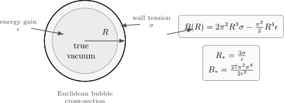
In the thin-wall limit, the Euclidean bounce is a nearly spherical bubble. The action balances wall tension, proportional to the area $2\pi^2R^3$, against the energy-density gain, proportional to the four-volume $\pi^2R^4/2$.

Vacuum persistence and the imaginary effective action

Fix the background, normalized initial and final vacuum states, regulator and boundary prescription. For finite initial and final times, let $U_J$ be the evolution operator with the source added as $+J\mathcal O$ in the action:

$$\begin{aligned} H_J(t)&=H_{\rm bg}(t)-\int d^{d-1}x\,J(t,\mathbf x)\mathcal O(\mathbf x),\\ U_J(t_f,t_i)&=T\exp\left[-i\int_{t_i}^{t_f}dt\,H_J(t)\right],\\ Z[J]&=\langle0_{\rm out}|U_J(t_f,t_i)|0_{\rm in}\rangle =e^{iW[J]}. \end{aligned}$$

Here $Z$ is the raw in–out amplitude; its zero-source value retains the background evolution. In scattering notation, after the appropriate asymptotic limits,

$$Z[0]=S_{00}.$$

Where $Z[0]\ne0$, the different, source-normalized functional is

$$\widehat Z[J]=\frac{Z[J]}{Z[0]} =e^{i(W[J]-W[0])}, \qquad \widehat Z[0]=1.$$

Choose the logarithm continuously on a region where $Z$ is nonzero. The normalization and the $+iJ\phi$ source derivative are explicit in Schwartz 2014, § 14.3, pp. 261–262, Eqs. (14.42)–(14.48). The canonical generating functional calls the raw functional $\mathcal Z$ and its normalized ratio $Z$; here the hat distinguishes that ratio because vacuum persistence requires the raw amplitude.

Division by $Z[J]$ normalizes an insertion in the background with that source. Thus $\delta W/\delta J=\langle\mathcal O\rangle_{J,\mathrm{in\text{–}out}}$, and differentiating again gives $i$ times the connected time-ordered two-point function. Equivalently, $iW=\log Z$ contains connected vacuum contributions, while their exponential contains all disconnected products Schwartz 2014, § 34.1.2, p. 738, Eqs. (34.17)–(34.20). If $C_a$ is the full amplitude of connected vacuum graph type $a$, its repeated disconnected copies sum as

$$Z[0]=\prod_a\sum_{n_a=0}^{\infty}\frac{C_a^{n_a}}{n_a!} =\exp\left(\sum_a C_a\right), \qquad iW[0]=\sum_a C_a.$$

This identity is order-by-order diagrammatic combinatorics; a metastable saddle sum additionally requires the decay prescription. In particular, vanishing connected contribution gives $Z=1$, not zero. Normalized source derivatives discard the constant $W[0]$, so $\widehat Z[0]$ cannot measure vacuum loss.

For a stable vacuum, $S_{00}$ is a phase after normalization. For an unstable vacuum, or for a background that can create real particles,

$$|S_{00}|<1.$$

Since

$$S_{00}=e^{iW[0]},$$

we have

$$|S_{00}|^2=e^{-2\operatorname{Im}W[0]}.$$

Therefore the probability that the initial vacuum remains the vacuum is

$$\boxed{ P_0=e^{-2\operatorname{Im}W[0]}. }$$

If the process is homogeneous and extensive in a spatial volume $\mathcal V$ over a long time $T$, write

$$W[0]=\mathcal V T\,\mathcal L_{\rm eff}.$$

Then the exact vacuum-loss exponent per spacetime volume is

$$\boxed{ \gamma_0 \equiv -\lim_{\mathcal VT\to\infty}{1\over\mathcal VT}\log P_0 =2\operatorname{Im}\mathcal L_{\rm eff}. }$$

For dilute, independently nucleated false-vacuum bubbles, $P_0=\exp[-(\Gamma/\mathcal V)\mathcal VT]$, so $\gamma_0=\Gamma/\mathcal V$. For pair production, however, $2\operatorname{Im}\mathcal L_{\rm eff}$ is the vacuum-persistence exponent. It need not equal the mean number of produced pairs per spacetime volume when multiple occupation of a mode is possible. Different sign conventions for $W$ move intermediate minus signs around, but $P_0=|Z|^2$ fixes the physical statement.

The diagram separates the connected sum from the raw amplitude it generates. Follow exponentiation before taking the modulus; replacing the raw amplitude by $\widehat Z$ would erase the survival probability.

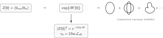
Connected vacuum contributions sum to $iW[0]=\log Z[0]$ and exponentiate into the raw amplitude $Z[0]$. For normalized in and out states, $\operatorname{Im}W[0]>0$ gives $P_0<1$. This is vacuum persistence, not the mean particle multiplicity. The diagram is schematic; the zero-contribution control gives $Z[0]=P_0=1$.

Perturbatively, an imaginary part appears when a diagram can go on shell. For example, a polarization bubble develops an absorptive part once the invariant momentum can create a pair,

$$q^2>4m^2.$$

Below threshold, the in–out vacuum may differ from the in-vacuum only by a phase. Above threshold, real quanta are produced. The vacuum-to-vacuum amplitude is no longer a pure phase, and the ordinary Feynman effective action is not the same as a causal expectation value in the produced state.

Weak-field ionization as a check

A simple quantum-mechanical estimate explains the common nonanalytic behavior $e^{-\operatorname{const}/|E|}$. Suppose a bound particle of binding energy $I$ is pulled apart by a weak constant external field $\mathcal E$. Near the exit region, approximate the barrier by

$$V(x)-E_{\rm bound}\simeq I-\mathcal F x, \qquad 0<x<{I\over\mathcal F}, \qquad \mathcal F\equiv|q\mathcal E|>0.$$

Here $q$ may be signed; $x$ is chosen in the escape direction and $\mathcal F$ is the positive force magnitude. The WKB exponent is

$$2\int_0^{I/\mathcal F}dx\,\sqrt{2M(I-\mathcal F x)}.$$

Evaluating the integral gives

$$2\sqrt{2M}\int_0^{I/\mathcal F}dx\,(I-\mathcal F x)^{1/2} = {4\sqrt{2M}\over3}{I^{3/2}\over\mathcal F}.$$

Thus

$$\boxed{ \Gamma_{\rm ion}\propto \exp\left[ -{4\sqrt{2M}\over3}{I^{3/2}\over\mathcal F} \right]. }$$

The important feature is not the detailed coefficient, which depends on the potential, but the essential singularity at zero field:

$$\Gamma_{\rm ion}\sim e^{-\operatorname{const}/|\mathcal E|}.$$

This is the same semiclassical pattern as Schwinger pair creation in a weak electric field and monopole-induced mass gaps proportional to $e^{-\operatorname{const}/g^2}$.

Stable amplitudes versus decaying amplitudes

For a stable vacuum,

$$\langle0|S(\infty,-\infty)|0\rangle=e^{i\alpha}.$$

Then the usual Feynman Green function may be written as a vacuum expectation value,

$$D_F(x,y)=\langle0|T\phi(x)\phi(y)|0\rangle,$$

without much danger. In the following Heisenberg notation the background evolution is absorbed into the in and out states, so their overlap denotes the raw $Z[0]$. The ordinary source-dependent Feynman path integral computes an in–out object:

$$G_{\rm in\text{–}out}(x,y)= { \langle0_{\rm out}|T\phi(x)\phi(y)|0_{\rm in}\rangle \over \langle0_{\rm out}|0_{\rm in}\rangle }.$$

When the vacuum decays or a background creates particles, $|0_{\rm out}\rangle$ is not just a phase times $|0_{\rm in}\rangle$. The in–out functional still computes transition amplitudes and the effective action, but it is not the same thing as a causal expectation value in the state prepared at $t=-\infty$.

For an operator $B(t)$, a true real-time expectation value has the schematic structure

$$\langle B(t)\rangle_{\rm in} = { \langle0_{\rm in}|S(-\infty,t)\,B(t)\,S(t,-\infty)|0_{\rm in}\rangle \over \langle0_{\rm in}|S(-\infty,t)S(t,-\infty)|0_{\rm in}\rangle }.$$

This evolves forward to the operator insertion and then backward. That forward–backward structure is the seed of the Schwinger–Keldysh, or closed-time-path, formalism. The next page builds that formalism systematically.

Summary

Instantons are classical solutions of Euclidean equations of motion. They arise because tunneling trajectories are not real classical solutions in real time, but become ordinary saddles after Wick rotation. For degenerate minima, an instanton connects one minimum to another and contributes factors such as $e^{-S_0}$ to tunneling amplitudes and energy splittings.

For a metastable false vacuum, the relevant Euclidean saddle is a bounce. It starts and ends at the false vacuum and reaches a turning point under the barrier. In quantum mechanics,

$$B=2\int_{x_f}^{x_t}dx\,\sqrt{2M\big(V(x)-V(x_f)\big)}.$$

In field theory,

$$B=S_E[\phi_B]-S_E[\phi_f].$$

The decay rate is

$$\Gamma\sim A e^{-B/\hbar}.$$

The imaginary part of the in–out effective action controls the probability that the vacuum channel remains empty:

$$P_0=|\langle0_{\rm out}|0_{\rm in}\rangle|^2 =e^{-2\operatorname{Im}W[0]}.$$

For dilute false-vacuum decay this exponent is the bubble-nucleation rate per spacetime volume. In a general particle-producing background it is a vacuum-persistence observable, not automatically the mean particle number. Once the vacuum can produce real particles, causal expectation values require the in–in formalism developed next.

Common pitfalls

Treating an instanton as a real-time trajectory. A Euclidean instanton is a saddle of the Wick-rotated path integral, not a real classical path through a forbidden region. It obeys classical motion in the inverted potential.

Mixing amplitudes and probabilities. A tunneling amplitude and a tunneling probability differ by a modulus square, so their leading exponents differ by a factor of two. State which quantity is being estimated before comparing WKB formulas.

Identifying every Euclidean saddle as a bounce. A double-well instanton connects different degenerate vacua and gives level mixing. A false-vacuum bounce returns to the same metastable configuration and has one negative mode that signals decay.

Dropping the return path. The quantum-mechanical bounce exponent is twice the one-way under-barrier action because the Euclidean solution goes to the turning point and returns. The one-way action is appropriate for the instanton amplitude between degenerate wells.

Calling $\operatorname{Im}W$ a violation of unitarity. A nonzero imaginary part means only that the vacuum final state has probability below one. The full evolution remains unitary after all final states are included.

Equating vacuum loss with mean multiplicity. The identity $-\log P_0=2\operatorname{Im}W$ is exact, but a mean number of produced particles is a different observable. They coincide only in special dilute Poisson limits.

Exercises

Exercise 1: Euclidean first integral

Starting from

$$S_E[x]=\int d\tau\,\left[{M\over2}(x')^2+V(x)\right],$$

show that a finite-action monotonic instanton connecting two degenerate minima $x_i<x_f$ with $V=0$ obeys

$${M\over2}(x')^2=V(x),$$

and derive

$$S_0=\int_{x_i}^{x_f}dx\,\sqrt{2MV(x)}.$$

Solution

The Euclidean equation of motion is

$$Mx''=V'(x).$$

Multiplying by $x'$ gives

$$Mx''x'=V'(x)x',$$

or

$${d\over d\tau}\left[{M\over2}(x')^2-V(x)\right]=0.$$

Thus

$${M\over2}(x')^2-V(x)=\mathcal E_E$$

is constant. For a finite-action trajectory beginning and ending at degenerate minima with $V=0$ and $x'\to0$, one has $\mathcal E_E=0$. Hence

$${M\over2}(x')^2=V(x).$$

For the increasing instanton specified in the question,

$$x'=\sqrt{{2V(x)\over M}}.$$

Then

$$S_0=\int d\tau\,\left[{M\over2}(x')^2+V(x)\right] =\int d\tau\,2V(x).$$

Using $d\tau=dx/x'$ gives

$$S_0=\int_{x_i}^{x_f}dx\,{2V(x)\over\sqrt{2V(x)/M}} =\int_{x_i}^{x_f}dx\,\sqrt{2MV(x)}.$$

The reverse anti-instanton has $x'<0$ and the same positive action. For either orientation one may write $S_0=\left|\int_{x_i}^{x_f}dx\,\sqrt{2MV(x)}\right|$; reversing the endpoints without also reversing the branch of $x'$ would give a spurious negative action.

Exercise 2: Quartic double-well instanton

For the quartic double well

$$V(x)={\lambda\over4}(x^2-a^2)^2, \qquad M=1,$$

verify that

$$x_I(\tau)=a\tanh{\omega(\tau-\tau_0)\over2}, \qquad \omega^2=2\lambda a^2,$$

solves the Euclidean equation and compute $S_0$.

Solution

Let

$$y={\omega(\tau-\tau_0)\over2}, \qquad x_I=a\tanh y.$$

Then

$$x_I'={a\omega\over2}\operatorname{sech}^2y,$$

and

$$x_I'' =-{a\omega^2\over2}\operatorname{sech}^2y\tanh y.$$

The potential derivative is

$$V'(x)=\lambda x(x^2-a^2).$$

For $x=a\tanh y$,

$$V'(x_I) =\lambda a\tanh y\,a^2(\tanh^2y-1) =-\lambda a^3\tanh y\,\operatorname{sech}^2y.$$

Since $\omega^2=2\lambda a^2$,

$$x_I''=V'(x_I),$$

so the solution is correct for $M=1$.

The action is

$$S_0=\int_{-a}^{a}dx\,\sqrt{2V(x)} =\int_{-a}^{a}dx\,\sqrt{\lambda\over2}(a^2-x^2),$$

where $a^2-x^2$ is positive in the interval. Therefore

$$S_0=\sqrt{\lambda\over2}\,{4a^3\over3} ={2\over3}a^2\omega.$$

Exercise 3: Bounce action and the return path

For a false vacuum $x_f$ with $V(x_f)=0$, choose the escape direction as increasing $x$ and let $x_t>x_f$ be the outer turning point with $V(x_t)=0$ and $V(x)>0$ between them. Show that the bounce action is

$$B=2\int_{x_f}^{x_t}dx\,\sqrt{2MV(x)}.$$

Why is there a factor of two?

Solution

The bounce starts at $x_f$, reaches $x_t$, and returns to $x_f$. Since $V(x_f)=0$ and $x'\to0$ at large $|\tau|$, the Euclidean energy is zero:

$${M\over2}(x')^2-V(x)=0.$$

On the outgoing half,

$$x'=\sqrt{{2V(x)\over M}},$$

so the half-bounce action is

$$B_{\rm half} =\int d\tau\,2V(x) =\int_{x_f}^{x_t}dx\,\sqrt{2MV(x)}.$$

On the returning half, $x'=-\sqrt{2V/M}$ and the integration endpoints reverse together. Its positive action is therefore the same. Hence

$$B=2B_{\rm half} =2\int_{x_f}^{x_t}dx\,\sqrt{2MV(x)}.$$

The factor of two is the Euclidean out-and-back motion. For escape toward smaller $x$, replace the oriented integral by its absolute value; the decay exponent remains positive.

Exercise 4: Weak-field ionization exponent

A bound particle of mass $M>0$ and binding energy $I>0$ escapes in the increasing-$x$ direction through the weak-field barrier. Define the positive force magnitude $\mathcal F=|q\mathcal E|>0$, allowing either sign of $q$:

$$V(x)-E_{\rm bound}=I-\mathcal F x, \qquad 0<x<{I\over\mathcal F}.$$

Use WKB to find the leading exponential dependence of the ionization rate on $|\mathcal E|$.

Solution

The WKB probability is

$$P\sim \exp\left[ -2\int_0^{I/\mathcal F}dx\, \sqrt{2M(I-\mathcal F x)} \right].$$

The integral is

$$\int_0^{I/\mathcal F}dx\,(I-\mathcal F x)^{1/2} ={1\over\mathcal F}\int_0^Idu\,u^{1/2} ={2\over3}{I^{3/2}\over\mathcal F}.$$

Thus

$$P\sim \exp\left[ -{4\sqrt{2M}\over3}{I^{3/2}\over\mathcal F} \right].$$

The decay rate has the same leading exponential dependence, multiplied by a prefactor depending on the bound-state normalization and attempt frequency.

Exercise 5: Vacuum persistence

Let

$$Z[0]=e^{iW[0]}.$$

Show that the no-decay probability is

$$P_0=e^{-2\operatorname{Im}W[0]}.$$

If $W[0]=\mathcal V T\mathcal L_{\rm eff}$, derive the vacuum-loss exponent

$$\gamma_0=2\operatorname{Im}\mathcal L_{\rm eff}.$$

Under what additional assumption may one identify $\gamma_0$ with a decay rate per spatial volume?

Solution

The vacuum persistence probability is

$$P_0=|Z[0]|^2=|e^{iW[0]}|^2.$$

Writing

$$W[0]=\operatorname{Re}W[0]+i\operatorname{Im}W[0],$$

gives

$$e^{iW[0]} =e^{i\operatorname{Re}W[0]-\operatorname{Im}W[0]}.$$

Therefore

$$P_0=e^{-2\operatorname{Im}W[0]}.$$

Define

$$\gamma_0=-{1\over\mathcal VT}\log P_0.$$

For an extensive effective action this gives

$$\gamma_0=2\operatorname{Im}\mathcal L_{\rm eff}.$$

If decay events are independent and occur at a constant rate per spatial volume, their number is Poisson distributed and the probability of no event is

$$P_0=e^{-(\Gamma/\mathcal V)\mathcal V T}.$$

Comparing exponents then gives

$${\Gamma\over\mathcal V}=2\operatorname{Im}\mathcal L_{\rm eff}.$$

Without the dilute independent-event assumption, the exact result remains the statement about $\gamma_0$; it need not equal a mean particle-production rate.

Exercise 6: Thin-wall critical bubble

In four Euclidean dimensions, the thin-wall bounce action for a bubble of radius $R$ is

$$B(R)=2\pi^2R^3\sigma-{\pi^2\over2}R^4\epsilon,$$

where $\sigma$ is the wall tension and $\epsilon$ is the false-minus-true vacuum energy density. Derive

$$R_*={3\sigma\over\epsilon}, \qquad B_*={27\pi^2\sigma^4\over2\epsilon^3}.$$

Solution

Extremize $B(R)$:

$${dB\over dR}=6\pi^2R^2\sigma-2\pi^2R^3\epsilon =2\pi^2R^2(3\sigma-R\epsilon).$$

The nonzero saddle has

$$R_*={3\sigma\over\epsilon}.$$

Substitute this into $B(R)$:

$$B_*=2\pi^2\left({3\sigma\over\epsilon}\right)^3\sigma -{\pi^2\over2}\left({3\sigma\over\epsilon}\right)^4\epsilon.$$

Thus

$$B_*={54\pi^2\sigma^4\over\epsilon^3} -{81\pi^2\sigma^4\over2\epsilon^3} ={27\pi^2\sigma^4\over2\epsilon^3}.$$

The large value of $B_*$ when $\epsilon$ is small expresses the intuitive fact that nearly degenerate vacua decay slowly: the critical bubble is large and expensive to nucleate.

References

• Callan, Curtis G., Jr., and Sidney Coleman. “Fate of the False Vacuum. II. First Quantum Corrections.” Physical Review D 16 (1977): 1762–1768. DOI.
• Coleman, Sidney. Aspects of Symmetry: Selected Erice Lectures. Cambridge University Press, 1985, ch. 7, § 2.4, pp. 279–282. DOI.
• Coleman, Sidney. “Fate of the False Vacuum: Semiclassical Theory.” Physical Review D 15 (1977): 2929–2936; erratum, Physical Review D 16 (1977): 1248. DOI.
• Coleman, Sidney, Vladimir Glaser, and André Martin. “Action Minima among Solutions to a Class of Euclidean Scalar Field Equations.” Communications in Mathematical Physics 58 (1978): 211–221. DOI.
• Schwartz, Matthew D. Quantum Field Theory and the Standard Model. Cambridge University Press, 2014, §§ 14.3 and 34.1.2. DOI.

Further reading

• Alexander M. Polyakov, Gauge Fields and Strings, Harwood Academic Publishers, 1987, Chapter 4.
• Jean Zinn-Justin, Quantum Field Theory and Critical Phenomena, 5th ed., Oxford University Press, 2021.