Vacuum Polarization and Gauge-Invariant Counterterms

The previous page organized QED as an effective field theory. Gauge invariance told us which local operators may appear, but it did not yet show how those operators are generated by loops. This page does the first serious calculation in that direction: the one-loop correction to the photon two-point function.

Physically, the photon does not propagate through an inert vacuum. Charged virtual quanta polarize the vacuum, and the long-distance electromagnetic field is the field after that polarization cloud has responded. Mathematically, this effect is encoded in the vacuum polarization tensor. Its ultraviolet-sensitive part is local and therefore renormalizes the coefficient of $F_{\mu\nu}F_{\mu\nu}$. Its nonlocal logarithmic part is the first appearance of the QED running charge.

The most important lesson is not the numerical coefficient, although we will compute it. The important lesson is structural:

$$\boxed{ q_\mu\Pi_{\mu\nu}(q)=0, \qquad \Pi_{\mu\nu}(q)=(q^2\delta_{\mu\nu}-q_\mu q_\nu)\Pi(q^2). }$$

The loop correction is transverse because gauge invariance forbids a photon mass and permits only gauge-invariant local counterterms. This remains true diagram by diagram only if the diagram set and regulator respect the gauge symmetry. Scalar QED is the cleanest place to see why the seagull vertex matters.

The quadratic photon effective action

Loop conventions used below. Most formulas on this page are Euclidean. We write

$$\int_q\equiv\int {d^4q\over(2\pi)^4}, \qquad q^2=q_\mu q_\mu, \qquad \delta_{\mu\nu}=\operatorname{diag}(1,1,1,1).$$

We use the gauge-field normalization introduced on the previous page,

$$\mathcal L_E={1\over4e_0^2}F_{\mu\nu}F_{\mu\nu}+\text{matter},$$

so the matter fields have unit positive charge in $D_\mu=\partial_\mu-iA_\mu$. In canonical normalization, $A_\mu=eA^{\rm can}_\mu$ and the same loop appears as the usual photon self-energy proportional to $e^2$.

What must be checked in any vacuum-polarization calculation

There are two independent checks on the answer.

First, the full tensor must be transverse:

$$q_\mu\Pi_{\mu\nu}(q)=0.$$

This check is sensitive to missing diagrams, especially the scalar-QED seagull term, and to regulators that break momentum-shift invariance.

Second, after transversality is established, the logarithmic coefficient multiplying $q^2\delta_{\mu\nu}-q_\mu q_\nu$ determines the running of $1/e^2$. Local finite constants can be changed by a subtraction convention; the coefficient of the large logarithm cannot be changed by such a convention at one loop.

The photon two-point function is most cleanly described through the effective action for a slowly varying background gauge field. To quadratic order,

$$\Gamma^{(2)}[A] ={1\over2}\int_q A_\mu(-q)K_{\mu\nu}(q)A_\nu(q).$$

At tree level,

$$K^{(0)}_{\mu\nu}(q) ={1\over e_0^2}(q^2\delta_{\mu\nu}-q_\mu q_\nu),$$

because

$${1\over4}\int d^4x\,F_{\mu\nu}F_{\mu\nu} ={1\over2}\int_q A_\mu(-q)(q^2\delta_{\mu\nu}-q_\mu q_\nu)A_\nu(q).$$

The loop correction is defined by

$$K_{\mu\nu}(q)=K^{(0)}_{\mu\nu}(q)+\Pi_{\mu\nu}(q)+\cdots.$$

Gauge invariance implies

$$\Gamma[A+\partial\alpha]=\Gamma[A].$$

In momentum space, the infinitesimal gauge variation is

$$\delta A_\mu(q)=iq_\mu\alpha(q).$$

Varying the quadratic effective action gives

$$0=\delta\Gamma^{(2)} =i\int_q \alpha(-q)q_\mu K_{\mu\nu}(q)A_\nu(q).$$

Since $\alpha$ and $A$ are arbitrary,

$$q_\mu K_{\mu\nu}(q)=0.$$

The tree kernel is already transverse, so the one-loop self-energy must satisfy

$$\boxed{q_\mu\Pi_{\mu\nu}(q)=0.}$$

Rotational invariance in Euclidean momentum space allows only

$$\Pi_{\mu\nu}(q)=A(q^2)\delta_{\mu\nu}+B(q^2)q_\mu q_\nu.$$

Transversality gives

$$A(q^2)+q^2B(q^2)=0,$$

so

$$\boxed{ \Pi_{\mu\nu}(q)=(q^2\delta_{\mu\nu}-q_\mu q_\nu)\Pi(q^2). }$$

A convenient projector for extracting the scalar function in $d$ Euclidean dimensions is

$$\Pi(q^2)={1\over(d-1)q^2} \left(\delta_{\mu\nu}-{q_\mu q_\nu\over q^2}\right)\Pi_{\mu\nu}(q),$$

provided the full tensor is already transverse. This projection is often the safest way to check signs and factors in explicit loop calculations.

The vacuum polarization tensor is the one-particle-irreducible correction to the photon two-point function. Gauge invariance forces it to be transverse, so its scalar content is a single function $\Pi(q^2)$ multiplying $q^2\delta_{\mu\nu}-q_\mu q_\nu$.

This equation is the local gauge-theory analog of a conservation law. If a calculation produces a term proportional to $\delta_{\mu\nu}\Lambda^2$ that survives at $q=0$, it has produced a photon mass term. Such a term is not allowed in QED. It either cancels after all gauge-required diagrams are included or signals that the regulator/subtraction has broken gauge invariance and must be repaired by a gauge-invariant prescription.

Gauge-invariant counterterms

Because the two-point kernel is transverse, its local ultraviolet-sensitive part must come from gauge-invariant local operators. The leading possibilities are

$$\Delta\Gamma_{\rm local}[A] =\int d^4x\, \left[ {\delta Z_A\over4}F_{\mu\nu}F_{\mu\nu} +{c_1\over\Lambda^2}(\partial_\rho F_{\mu\nu})(\partial_\rho F_{\mu\nu}) +{c_2\over\Lambda^4}F^4+ \cdots \right].$$

The first term renormalizes $1/e^2$. The second is a higher-derivative photon operator and contributes to the two-point function with extra powers of $q^2/\Lambda^2$. The $F^4$ terms affect four-photon scattering and begin the Euler–Heisenberg effective action if charged matter is integrated out.

The forbidden term is

$${1\over2}m_A^2A_\mu A_\mu.$$

It would contribute

$$K_{\mu\nu}(q)\supset m_A^2\delta_{\mu\nu},$$

which is not transverse. A gauge-invariant regulator makes this absence automatic; a careless hard cutoff can obscure it because shifts of loop momentum are not innocent in divergent integrals.

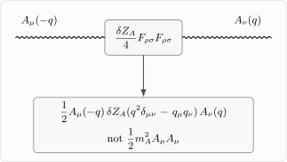
The local counterterm $\delta(1/e^2)F_{\mu\nu}F_{\mu\nu}/4$ contributes exactly the transverse two-point kernel. A photon mass would instead give a non-transverse $\delta_{\mu\nu}$ term and is forbidden by gauge invariance.

It is useful to separate three things that often get conflated:

1. The tensor structure is fixed by gauge invariance.
2. The logarithmic coefficient is computed by a loop integral and determines the one-loop beta function.
3. The finite local piece depends on the subtraction convention used to define the renormalized coupling.

The tensor structure is exact. The coefficient below is a one-loop result.

Scalar QED as the clean test case

Consider one charged complex scalar in Euclidean signature,

$$\mathcal L_E ={1\over4e_0^2}F_{\mu\nu}F_{\mu\nu} +(D_\mu\phi)^*(D_\mu\phi)+m^2\phi^*\phi+\lambda(\phi^*\phi)^2, \qquad D_\mu=\partial_\mu-iA_\mu.$$

Expanding the covariant kinetic term gives

$$(D_\mu\phi)^*(D_\mu\phi) =\partial_\mu\phi^*\partial_\mu\phi -iA_\mu(\phi\partial_\mu\phi^*-\phi^*\partial_\mu\phi) +A_\mu A_\mu\phi^*\phi.$$

The term linear in $A_\mu$ gives the derivative photon-scalar-scalar vertex. The term quadratic in $A_\mu$ gives the two-photon seagull vertex. Gauge invariance fixes the two together; keeping the bubble while omitting the seagull is not an approximation to scalar QED, it is a different and non-gauge-invariant theory.

The one-loop quadratic effective action receives two contributions:

$$\Pi^{(s)}_{\mu\nu}(q) =-\int_k {(2k+q)_\mu(2k+q)_\nu \over (k^2+m^2)((k+q)^2+m^2)} +2\delta_{\mu\nu}\int_k{1\over k^2+m^2}.$$

The first term is the scalar loop with two derivative vertices; the second is the seagull. The sign of the one-photon vertex depends on the charge convention, but the two-vertex bubble depends on its square; the seagull coefficient is fixed by the same covariant kinetic term. The sign convention above is chosen so that $\Pi_{\mu\nu}$ is the addition to the inverse photon kernel $K_{\mu\nu}$ in $\Gamma^{(2)}$.

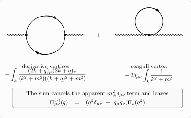
In scalar QED the vacuum polarization is the sum of the derivative-vertex bubble and the seagull diagram. The quadratic divergence cancels in the gauge-invariant sum, leaving a transverse logarithmic correction to the Maxwell term.

At $q=0$, the expression must vanish. Indeed, using a gauge-invariant regulator or dimensional regularization,

$$0=\int_k{\partial\over\partial k_\mu} \left({k_\nu\over k^2+m^2}\right) =\delta_{\mu\nu}\int_k{1\over k^2+m^2} -2\int_k{k_\mu k_\nu\over(k^2+m^2)^2}.$$

Therefore

$$-4\int_k{k_\mu k_\nu\over(k^2+m^2)^2} +2\delta_{\mu\nu}\int_k{1\over k^2+m^2}=0.$$

This is the cancellation of the apparent photon mass term. The cancellation is not a numerical accident; it is the Ward identity showing up inside the loop integral.

Extracting the logarithm

To get the coefficient of the Maxwell counterterm, combine denominators by

$${1\over ab}=\int_0^1 dx\,{1\over[xa+(1-x)b]^2}.$$

For

$$a=k^2+m^2, \qquad b=(k+q)^2+m^2,$$

shift the loop momentum to

$$\ell=k+(1-x)q,$$

so the denominator becomes

$$(\ell^2+\Delta)^2, \qquad \Delta=m^2+x(1-x)q^2.$$

After the angular average over $\ell$ and after adding the seagull term, the non-transverse pieces cancel. The remaining gauge-invariant part is

$$\Pi^{(s)}_{\mu\nu}(q) =(q^2\delta_{\mu\nu}-q_\mu q_\nu)\Pi_s(q^2),$$

where the logarithmic part is

$$\boxed{ \Pi_s(q^2) ={1\over16\pi^2}\int_0^1 dx\,(1-2x)^2 \log {\Lambda^2\over m^2+x(1-x)q^2} +\text{finite local convention}. }$$

Here $\Lambda$ is a short-distance cutoff used only to display the logarithm. In a subtraction scheme such as dimensional regularization with minimal subtraction, the same information appears as a pole and a subtraction scale $\mu$.

For momenta large compared with the scalar mass but still below the microscopic cutoff,

$$q^2\gg m^2,$$

the coefficient of the large logarithm is determined by

$$\int_0^1 dx\,(1-2x)^2={1\over3}.$$

Thus

$$\boxed{ \Pi_s(q^2) ={1\over3}{1\over16\pi^2} \log {\Lambda^2\over q^2} +\text{finite terms}. }$$

This is the coefficient visible in the effective Maxwell action. In momentum space,

$$\Gamma^{(2)}[A] ={1\over2}\int_q A_\mu(-q)(q^2\delta_{\mu\nu}-q_\mu q_\nu)A_\nu(q) \left[ {1\over e_0^2}+{1\over48\pi^2}\log {\Lambda^2\over q^2}+\cdots \right].$$

Equivalently,

$${1\over e^2(q)} ={1\over e_0^2}+{1\over48\pi^2}\log {\Lambda^2\over q^2}+\cdots,$$

or

$$\boxed{ e^2(q)= {e_0^2\over 1+{e_0^2\over48\pi^2}\log(\Lambda^2/q^2)+\cdots }. }$$

At lower momenta, $q^2\ll m^2$, the logarithm is cut off by the scalar mass:

$$\Pi_s(q^2) ={1\over48\pi^2}\log{\Lambda^2\over m^2}+O(q^2/m^2).$$

This is decoupling in its simplest form. Once the charged particle is too heavy to be produced or resolved, its remaining low-energy effect is a local renormalization of $F^2$ plus higher-derivative operators suppressed by powers of $q^2/m^2$.

Spinor QED comparison

A Dirac fermion gives the same tensor structure but a different coefficient. In the rescaled normalization, integrating out one Dirac fermion gives

$$\Gamma_{\rm 1-loop}^{(f)}[A] =-\operatorname{Tr}\log(D\!\!\!/+m), \qquad D\!\!\!/\equiv\gamma_\mu D_\mu,$$

where the minus sign is the Grassmann sign. Squaring the Dirac operator displays two ingredients:

$$(D\!\!\!/)^2 =D^2-{i\over2}\sigma_{\mu\nu}F_{\mu\nu}, \qquad \sigma_{\mu\nu}={1\over2}[\gamma_\mu,\gamma_\nu]$$

in Euclidean conventions up to the standard convention-dependent factors of $i$. The first term resembles the scalar covariant Laplacian; the second is the spin coupling to the background field.

The final one-loop logarithm for one unit-charge Dirac fermion is

$$\boxed{ \Pi_f(q^2) ={4\over3}{1\over16\pi^2} \log {\Lambda^2\over q^2}+\cdots. }$$

Thus, for $N_f$ Dirac fermions and $N_s$ complex scalars of unit charge,

$${1\over e^2(q)} ={1\over e_0^2} +{1\over16\pi^2} \left({4\over3}N_f+{1\over3}N_s\right) \log{\Lambda^2\over q^2} +\cdots.$$

Differentiating with respect to $\mu$ gives the familiar one-loop QED beta function,

$$\boxed{ \beta(e)=\mu{de\over d\mu} ={e^3\over16\pi^2} \left({4\over3}N_f+{1\over3}N_s\right)+O(e^5). }$$

The positive sign means that QED charge increases toward shorter distances. Equivalently, $1/e^2(q)$ increases as we run toward longer distances. The physical interpretation is screening: a test charge is surrounded by a polarization cloud of opposite charge, so a distant observer sees a reduced charge. The next pages turn this statement into the broader comparison between screening in QED and antiscreening in non-Abelian gauge theory.

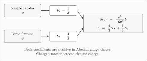
Charged scalars and Dirac fermions both screen Abelian charge. Their one-loop contributions differ by spin and statistics: a complex scalar contributes $1/3$, while a Dirac fermion contributes $4/3$ to the coefficient multiplying $e^3/(16\pi^2)$.

What is local and what is nonlocal

The expression

$$\Pi_s(q^2)\sim {1\over48\pi^2}\log{\Lambda^2\over q^2}$$

contains two different pieces of physics:

$$\log{\Lambda^2\over q^2} =\log{\Lambda^2\over\mu^2}+\log{\mu^2\over q^2}.$$

The first term is local. It is absorbed into the definition of the renormalized coefficient $1/e^2(\mu)$. The second term is nonlocal in position space. It is the physical logarithmic dependence of the two-point function on momentum.

This split is arbitrary because $\mu$ is arbitrary, but the sum is not. Changing $\mu$ moves information between the coupling and the explicit logarithm. The Callan–Symanzik equation is the statement that this move is a change of coordinates, not a change of physics.

In a Wilsonian language, integrating out a momentum shell changes the coefficient of $F^2$:

$$\Delta\!\left({1\over e^2}\right) ={1\over16\pi^2} \left({4\over3}N_f+{1\over3}N_s\right)\Delta\log{\Lambda^2\over q^2}$$

for the active charged fields in the shell. In a renormalized perturbation theory language, the same coefficient appears as the beta function. Same physics, different bookkeeping.

Summary

Vacuum polarization is the one-loop correction to the photon two-point function caused by charged quantum fluctuations. Gauge invariance forces the correction to be transverse:

$$\Pi_{\mu\nu}(q)=(q^2\delta_{\mu\nu}-q_\mu q_\nu)\Pi(q^2).$$

Therefore the leading local counterterm is $F_{\mu\nu}F_{\mu\nu}$, not $A_\mu A_\mu$. In scalar QED the derivative bubble and the seagull diagram are both required; their sum cancels the apparent photon mass and leaves a logarithmic correction,

$$\Pi_s(q^2)={1\over48\pi^2}\log{\Lambda^2\over q^2}+\cdots$$

for one charged complex scalar. A Dirac fermion gives four times the scalar coefficient in the Abelian beta-function normalization:

$$\Pi_f(q^2)={4\over3}{1\over16\pi^2}\log{\Lambda^2\over q^2}+\cdots.$$

In the rescaled gauge-field convention, these loops renormalize the coefficient of $F^2$:

$${1\over e^2(q)}={1\over e_0^2}+\Pi(q^2).$$

The positive QED beta function is the scale-space expression of screening.

Common pitfalls

Inferring a photon mass from one divergent diagram. Gauge invariance constrains the sum of diagrams and the regulator. In scalar QED, the seagull is essential.

Shifting a divergent integral without checking the regulator. Do not freely shift loop momenta in a hard-cutoff integral unless the regulator respects the symmetry. Dimensional regularization and gauge-invariant Pauli–Villars schemes preserve the Ward identity more transparently.

Mixing photon normalizations. In canonical normalization, the one-loop self-energy contains explicit factors of $e^2$. In the rescaled normalization used here, charged fields have unit charge and loops directly correct $1/e^2$.

Treating every local term as observable. The finite part of the $F^2$ counterterm depends on the subtraction scheme; the one-loop logarithmic coefficient and the transversality condition are the robust data.

Mistaking transversality for a vanishing two-point function. Transversality means that the tensor is orthogonal to $q_\mu$ on its gauge index, not that the tensor itself vanishes.

Exercises

Exercise 1 — The Maxwell quadratic kernel

Show that

$${1\over4}\int d^4x\,F_{\mu\nu}F_{\mu\nu} ={1\over2}\int_q A_\mu(-q)(q^2\delta_{\mu\nu}-q_\mu q_\nu)A_\nu(q).$$

Solution

Use

$$A_\mu(x)=\int_q e^{iq\cdot x}A_\mu(q),$$

so

$$F_{\mu\nu}(q)=i(q_\mu A_\nu(q)-q_\nu A_\mu(q)).$$

Then

$$F_{\mu\nu}(-q)F_{\mu\nu}(q) =(q_\mu A_\nu(-q)-q_\nu A_\mu(-q)) (q_\mu A_\nu(q)-q_\nu A_\mu(q)).$$

Expanding and relabeling dummy indices gives

$$F_{\mu\nu}(-q)F_{\mu\nu}(q) =2q^2A_\mu(-q)A_\mu(q)-2q_\mu q_\nu A_\mu(-q)A_\nu(q).$$

Therefore

$${1\over4}\int_q F_{\mu\nu}(-q)F_{\mu\nu}(q) ={1\over2}\int_q A_\mu(-q)(q^2\delta_{\mu\nu}-q_\mu q_\nu)A_\nu(q).$$

Exercise 2 — Transverse tensor decomposition

Assume rotational invariance gives

$$\Pi_{\mu\nu}(q)=A(q^2)\delta_{\mu\nu}+B(q^2)q_\mu q_\nu.$$

Use $q_\mu\Pi_{\mu\nu}=0$ to derive the transverse form of $\Pi_{\mu\nu}$.

Solution

Contracting with $q_\mu$ gives

$$q_\mu\Pi_{\mu\nu}(q) =\left(A(q^2)+q^2B(q^2)\right)q_\nu.$$

For this to vanish for arbitrary nonzero $q_\nu$, we need

$$A(q^2)=-q^2B(q^2).$$

Hence

$$\Pi_{\mu\nu}(q)=B(q^2)(q_\mu q_\nu-q^2\delta_{\mu\nu}).$$

If we define $\Pi(q^2)=-B(q^2)$, then

$$\Pi_{\mu\nu}(q)=(q^2\delta_{\mu\nu}-q_\mu q_\nu)\Pi(q^2).$$

The sign is a convention absorbed into the scalar function $\Pi(q^2)$.

Exercise 3 — Bubble–seagull cancellation

Verify explicitly that the scalar QED bubble plus seagull has no photon mass term at $q=0$:

$$\Pi^{(s)}_{\mu\nu}(0) =-4\int_k{k_\mu k_\nu\over(k^2+m^2)^2} +2\delta_{\mu\nu}\int_k{1\over k^2+m^2}=0.$$

Use integration by parts in a regulator that discards surface terms.

Solution

Consider

$$0=\int_k{\partial\over\partial k_\mu} \left({k_\nu\over k^2+m^2}\right).$$

Differentiating gives

$${\partial\over\partial k_\mu} \left({k_\nu\over k^2+m^2}\right) ={\delta_{\mu\nu}\over k^2+m^2} -{2k_\mu k_\nu\over(k^2+m^2)^2}.$$

Therefore

$$\delta_{\mu\nu}\int_k{1\over k^2+m^2} =2\int_k{k_\mu k_\nu\over(k^2+m^2)^2}.$$

Multiplying this identity by $2$ gives

$$2\delta_{\mu\nu}\int_k{1\over k^2+m^2} =4\int_k{k_\mu k_\nu\over(k^2+m^2)^2}.$$

Substituting into $\Pi^{(s)}_{\mu\nu}(0)$ gives zero. This is the diagrammatic cancellation of the forbidden photon mass.

Exercise 4 — The complex-scalar logarithm

Compute

$$\int_0^1 dx\,(1-2x)^2$$

and use it to derive the coefficient of the leading scalar QED logarithm.

Solution

Expand the square:

$$(1-2x)^2=1-4x+4x^2.$$

Then

$$\int_0^1 dx\,(1-2x)^2 =1-4\cdot{1\over2}+4\cdot{1\over3} =1-2+{4\over3} ={1\over3}.$$

The logarithmic part of the scalar vacuum polarization is

$$\Pi_s(q^2) ={1\over16\pi^2}\int_0^1 dx\,(1-2x)^2 \log{\Lambda^2\over q^2}+\cdots.$$

Using the integral gives

$$\Pi_s(q^2) ={1\over3}{1\over16\pi^2} \log{\Lambda^2\over q^2}+\cdots ={1\over48\pi^2}\log{\Lambda^2\over q^2}+\cdots.$$

Exercise 5 — Beta function from the inverse charge

Suppose

$${1\over e^2(\mu)}={1\over e^2(\Lambda)}+{b\over16\pi^2}\log{\Lambda^2\over\mu^2}.$$

Show that

$$\beta(e)=\mu{de\over d\mu}={b e^3\over16\pi^2}$$

to one-loop order.

Solution

Differentiate with respect to $\log\mu$ at fixed bare coupling:

$${d\over d\log\mu}{1\over e^2(\mu)} ={b\over16\pi^2}{d\over d\log\mu}\left(\log\Lambda^2-\log\mu^2\right) =-{2b\over16\pi^2}.$$

On the other hand,

$${d\over d\log\mu}{1\over e^2} =-{2\over e^3}{de\over d\log\mu} =-{2\beta(e)\over e^3}.$$

Equating the two expressions gives

$$-{2\beta(e)\over e^3}=-{2b\over16\pi^2},$$

and therefore

$$\beta(e)={b e^3\over16\pi^2}.$$

For one complex scalar, $b=1/3$. For one Dirac fermion, $b=4/3$.

Further reading

• Coleman, Sidney. Lectures of Sidney Coleman on Quantum Field Theory. Edited by Bryan Gin-ge Chen, David Derbes, David Griffiths, Brian Hill, Richard Sohn, and Yuan-Sen Ting. World Scientific, 2019. See the lectures on electrodynamics, renormalization, and Ward identities.
• Schwartz, Matthew D. Quantum Field Theory and the Standard Model. Cambridge University Press, 2014, chapters 16, 19, and 23.
• Srednicki, Mark. Quantum Field Theory. Cambridge University Press, 2007, sections 61, 65, and 66.
• Weinberg, Steven. The Quantum Theory of Fields, Volume I: Foundations. Cambridge University Press, 1995, chapters 11–12; and Volume II: Modern Applications. Cambridge University Press, 1996, chapter 18.
• Zee, A. Quantum Field Theory in a Nutshell. 2nd ed. Princeton University Press, 2010, part III.