Commutators, Currents, and Ward Identities

Vacuum commutator expectations and current Ward identities describe different singularities of correlation functions: the former compare Lorentzian operator orderings, while the latter determine contact terms at transformed insertions. This lesson first uses an exact scalar conformal two-point function, then derives equations of motion inside a stable regulated Euclidean integral and obtains the current identities. The final conditional pole argument introduces spontaneous breaking of a continuous global symmetry.

The current records how the action changes when a global symmetry parameter is allowed to vary in space. In a correlation function this produces contact terms at the charged insertions. The localized parameter is an arbitrary admissible infinitesimal test function; it need not vary slowly.

The bridge between the two themes is locality. Commutators tell us where an operator can causally respond. Ward identities tell us how a local symmetry variation is distributed among operator insertions. Both are statements about singularities of correlation functions.

Required background. Lesson 17 supplies ordered vacuum boundary values, distributional light-cone limits and the distinction between a raw time-ordered correlator and causal response.

Commutators as discontinuities

Dimensions, boundary values, and charge generators

We write $D$ for spacetime dimension and $d=D-1$ for the number of spatial dimensions. Thus equal-time canonical relations contain $\delta^{(d)}(\mathbf x-\mathbf y)$, while Euclidean Ward identities contain $d^D x$ and $\delta^{(D)}(x-x_k)$.

For Lorentzian formulas we write

$$\rho=\mathbf x^2-t^2.$$

Thus spacelike separation has $\rho>0$, while timelike separation has $\rho<0$. Wightman boundary values are written as

$$W_+(t,\mathbf x)=\langle0|O(t,\mathbf x)O(0)|0\rangle, \qquad W_-(t,\mathbf x)=\langle0|O(0)O(t,\mathbf x)|0\rangle.$$

For Ward identities we mostly use Euclidean path-integral notation,

$$Z=\int D\phi\,e^{-S[\phi]}.$$

An infinitesimal internal symmetry acts as

$$\delta \Phi_k=\alpha(x)R_k\Phi_k.$$

For a $U(1)$ field of charge $e_k$, $R_k=i e_k$ in the convention $\Phi_k\mapsto e^{i e_k\alpha}\Phi_k$. Different authors absorb the factor of $i$ into the generator; the contact-term structure is independent of this bookkeeping.

Consider a nonidentity Hermitian scalar primary in a unitary conformal vacuum, with admissible scaling dimension $\Delta$ and positive normalization $C_O$. Its exact Euclidean two-point function is

$$\langle O(x_E)O(0)\rangle={C_O\over (x_E^2)^\Delta}.$$

This is a statement at all noncoincident separations in the exact CFT. A short-distance asymptote in a more general theory cannot determine a finite-separation correlator. For example, in $D>2$ the leading short-distance power of a massive free scalar is massless, but it cannot be its exact correlator: away from coincidence the massive Klein–Gordon operator acting on the massless power leaves $m^2W_+^{(0)}\ne0$.

After analytic continuation to Lorentzian time, the two Wightman orderings are distributional boundary values on opposite sides of the light-cone singularity:

$$W_+(t,\mathbf x) ={C_O\over \left(\mathbf x^2-(t-i0)^2\right)^\Delta} ={C_O\over \left(\rho+i0\,\operatorname{sgn}t\right)^\Delta},$$

and

$$W_-(t,\mathbf x) ={C_O\over \left(\mathbf x^2-(t+i0)^2\right)^\Delta} ={C_O\over \left(\rho-i0\,\operatorname{sgn}t\right)^\Delta}.$$

Therefore

$$\langle0|[O(t,\mathbf x),O(0)]|0\rangle =W_+(t,\mathbf x)-W_-(t,\mathbf x).$$

See Gillioz 2023, arXiv v3, § 3.4, pp. 27–29 (PDF). His ordering is $W_G(x)=\langle\phi(0)\phi(x)\rangle$, so the present $W_+(x)=W_G(-x)$. With his squared interval equal to $\rho$, this translation gives the displayed lower-time prescription and the discontinuity sign below.

For spacelike separation, $\rho>0$, the two boundary values are the same. The commutator vanishes:

$$\boxed{ \langle0|[O(t,\mathbf x),O(0)]|0\rangle=0 \qquad (\mathbf x^2>t^2). }$$

This is the two-point, vacuum-expectation version of causality. Microcausality is the stronger operator statement $[O(x),O(0)]=0$ at spacelike separation (or the graded version for fermionic fields).

The branch-cut and causal-support diagram in Lesson 17 shows how the two banks interchange when time changes sign, and why spacelike values agree.

For non-integer $\Delta$, the timelike discontinuity is easy to compute. When $\rho<0$, write $\rho=-|\rho|$. On the principal branch,

$$(\rho+i0)^{-\Delta}=|\rho|^{-\Delta}e^{-i\pi\Delta}, \qquad (\rho-i0)^{-\Delta}=|\rho|^{-\Delta}e^{+i\pi\Delta}.$$

Taking into account the factor $\operatorname{sgn}t$ in the boundary prescription gives

$$\boxed{ W_+(t,\mathbf x)-W_-(t,\mathbf x) =-2iC_O\sin(\pi\Delta)\,\operatorname{sgn}t\, {\theta(t^2-\mathbf x^2)\over (t^2-\mathbf x^2)^\Delta} }$$

for non-integer $\Delta$, away from the light cone.

The negative sign follows from the displayed ordering and principal branch. Globally the result means the distribution inherited from the analytic Wightman boundary values, including the light cone; for $\Delta\ge1$, the power times the step function is not independently an ordinary locally integrable function there. Its support satisfies

$$\operatorname{supp}\langle[O(x),O(0)]\rangle \subseteq \{x: t^2\ge \mathbf x^2\}.$$

For integer $\Delta$, the factor $\sin(\pi\Delta)$ seems to vanish. This does not mean that the commutator vanishes. Instead the discontinuity collapses to derivatives of delta functions on the light cone. For example,

$${1\over \rho+i0}-{1\over \rho-i0}=-2\pi i\,\delta(\rho).$$

This is why the free massless scalar in four dimensions has a commutator supported on the light cone rather than throughout the timelike interior.

Equal-time algebra and the ultraviolet cutoff

A continuum theory can describe the long-distance limit of lattice degrees of freedom. For lattice spacing $a$, the ultraviolet cutoff is of order

$$\Lambda_{\mathrm{UV}}\sim {1\over a}.$$

A continuum scaling law must be restricted to its scaling regime, with separations much larger than $a$ and the correlation length controlled when it is finite. Canonical equal-time commutators are local. For a scalar with the standard kinetic normalization, their singular support lies at coincident spatial points:

$$[\phi(t,\mathbf x),\phi(t,\mathbf y)]=0,$$

and

$$[\phi(t,\mathbf x),\pi(t,\mathbf y)]=i\delta^{(d)}(\mathbf x-\mathbf y), \qquad \pi=\dot\phi.$$

The delta function is the continuum limit of a sharply localized lattice kernel. It is not resolved by the long-distance CFT power law. This is the same warning in a different language: the normalization and possible local improvement of contact terms are ultraviolet data that survive as distributions.

The mechanical analogy is useful but must be handled carefully. For a single nonlinear oscillator,

$$\ddot x+\omega^2x+\lambda x^3=0,$$

the initial data $x(0),\dot x(0)$ determine $x(t)$. For a field, the equation of motion propagates operator data from one time slice to another. But products of fields at the same point are singular, so the equation of motion is an operator identity only after specifying renormalized composite operators and contact terms.

A stable regulated Schwinger–Dyson identity

An explicit finite regulator makes the integration-by-parts premise precise. Take real field variables on a finite periodic Euclidean lattice and the normalized weight $e^{-S_a}/Z_a$, where

$$\begin{aligned} S_a&=a^D\sum_n\left[ \frac12\sum_{\mu=1}^D\left(\frac{\phi_{n+\hat\mu}-\phi_n}{a}\right)^2 +\frac{m_0^2}{2}\phi_n^2+\frac{\lambda_0}{4!}\phi_n^4\right],\\ &\hspace{1em}\lambda_0>0,\qquad m_0^2\ge0. \end{aligned}$$

There are finitely many ordinary real integrals. The positive quartic term dominates every polynomial insertion at large field values, so the integral of $\partial_{\phi_n}(e^{-S_a}\mathcal O)$ has zero field-space boundary flux. Define

$$\begin{aligned} E_{a,n}&=a^{-D}\frac{\partial S_a}{\partial\phi_n} =-\Delta_a\phi_n+m_0^2\phi_n+\frac{\lambda_0}{6}\phi_n^3,\\ \Delta_a\phi_n&=\frac1{a^2}\sum_\mu (\phi_{n+\hat\mu}+\phi_{n-\hat\mu}-2\phi_n). \end{aligned}$$

Ordinary integration by parts now proves the exact finite-dimensional identity

$$\langle E_{a,n}\mathcal O\rangle_a =a^{-D}\left\langle\frac{\partial\mathcal O}{\partial\phi_n}\right\rangle_a.$$

For a product of lattice fields the contacts are $a^{-D}\delta_{n,n_k}$, with the corresponding insertion omitted. On a bounded field-integration domain, any nonzero boundary flux must instead be retained. A real cubic action over the full real contour does not meet this positive-integral premise: its constant-field direction is unbounded below.

The continuum Schwinger–Dyson notation summarizes the corresponding identity after a continuum/composite prescription has been supplied. For a scalar field and a product of insertions $\mathcal O[\phi]$,

$$0=\int D\phi\,{\delta\over\delta\phi(x)} \left(e^{-S[\phi]}\mathcal O[\phi]\right).$$

Therefore

$$\boxed{ \left\langle {\delta S\over\delta\phi(x)}\mathcal O\right\rangle =\left\langle {\delta\mathcal O\over\delta\phi(x)}\right\rangle. }$$

For

$$\mathcal O=\phi(x_1)\cdots\phi(x_n),$$

this becomes

$$\left\langle {\delta S\over\delta\phi(x)}\phi(x_1)\cdots\phi(x_n)\right\rangle =\sum_{k=1}^n\delta^{(D)}(x-x_k) \left\langle\phi(x_1)\cdots\widehat{\phi(x_k)}\cdots\phi(x_n)\right\rangle,$$

where the hat means omission. Away from $x=x_k$, the classical-looking equation of motion is valid inside correlation functions. At $x=x_k$, the contact terms are part of the identity.

For the quartic example, the formal continuum expressions are

$$S_E=\int d^D x\left[\frac12(\partial\phi)^2+\frac{m_0^2}{2}\phi^2+\frac{\lambda_0}{4!}\phi^4\right],$$

then

$$\frac{\delta S_E}{\delta\phi(x)}=-\partial^2\phi(x)+m_0^2\phi(x)+\frac{\lambda_0}{6}\phi^3(x),$$

so the equation

$$\partial^2\phi=m_0^2\phi+\frac{\lambda_0}{6}\phi^3$$

is the bare regulated equation, not a pointwise equality of unrenormalized continuum products. Regulator removal requires counterterms and defined composite insertions; the renormalized equation and its contacts must be obtained together. The finite integral does not by itself prove a continuum limit. Compare the field-shift derivation in Schwartz 2014, § 14.7.1, pp. 273–274, and § 14.7.2, p. 275: his Lorentzian weight gives different factors of $i$, while the Euclidean sign here follows directly from differentiating $e^{-S_E}$.

Noether currents from localizing a symmetry

Suppose the action is invariant under a constant internal transformation

$$\delta\Phi_k=\alpha R_k\Phi_k, \qquad \alpha=\text{constant}.$$

For an action depending on fields and their first derivatives, promote $\alpha$ to a smooth compactly supported function $\alpha(x)$. To first order in its amplitude, the variation is

$$\delta S=\int d^D x\,J_\mu(x)\partial_\mu\alpha(x).$$

Integrating by parts gives

$$\delta S=-\int d^D x\,\alpha(x)\partial_\mu J_\mu(x),$$

with no boundary term for this parameter. Since constant $\alpha$ is an exact symmetry, only derivatives of $\alpha$ appear. Their coefficient is the Noether current. Higher-derivative actions can first produce higher derivatives of the parameter; integration by parts then identifies a current, with its usual improvement freedom.

For a complex scalar with Euclidean action

$$S=\int d^D x\left(\partial_\mu\phi^*\partial_\mu\phi+V(|\phi|^2)\right),$$

the global $U(1)$ transformation is

$$\phi\mapsto e^{i\alpha}\phi, \qquad \phi^*\mapsto e^{-i\alpha}\phi^*.$$

For local $\alpha(x)$,

$$\delta\phi=i\alpha\phi, \qquad \delta\phi^*=-i\alpha\phi^*.$$

The variation of the kinetic term is

$$\delta S =\int d^D x\,i\left(\phi\partial_\mu\phi^*-\phi^*\partial_\mu\phi\right)\partial_\mu\alpha.$$

Thus one convenient Euclidean convention is

$$J_\mu=i\left(\phi\partial_\mu\phi^*-\phi^*\partial_\mu\phi\right).$$

The conservation equation

$$\partial_\mu J_\mu=0$$

holds as an operator statement away from insertions and, equivalently, as a Ward identity inside correlators.

Ward identities in position space

Let

$$\mathcal O=\Phi_1(x_1)\Phi_2(x_2)\cdots\Phi_n(x_n).$$

Use a symmetry-preserving regulator and measure, an admissible compactly supported parameter, and no anomalous Jacobian. Perform the local change of integration variables. The regulated integral does not change:

$$0=\int D\Phi\,\delta\left(e^{-S}\mathcal O\right) =\left\langle\delta\mathcal O\right\rangle- \left\langle\mathcal O\,\delta S\right\rangle.$$

Using

$$\delta S=-\int d^D x\,\alpha(x)\partial_\mu J_\mu(x),$$

and

$$\delta\mathcal O=\sum_{k=1}^n\alpha(x_k) \Phi_1(x_1)\cdots R_k\Phi_k(x_k)\cdots\Phi_n(x_n),$$

we obtain

$$0=\int d^D x\,\alpha(x) \left[ \partial_\mu\langle J_\mu(x)\mathcal O\rangle +\sum_{k=1}^n\delta^{(D)}(x-x_k) \langle\Phi_1\cdots R_k\Phi_k\cdots\Phi_n\rangle \right].$$

Because $\alpha(x)$ is arbitrary,

$$\boxed{ \partial_\mu\langle J_\mu(x)\Phi_1(x_1)\cdots\Phi_n(x_n)\rangle =-\sum_{k=1}^n\delta^{(D)}(x-x_k) \langle\Phi_1\cdots R_k\Phi_k\cdots\Phi_n\rangle. }$$

For $U(1)$ charges $e_k$, with $R_k=i e_k$, this is

$$\boxed{ \partial_\mu\langle J_\mu(x)\Phi_1(x_1)\cdots\Phi_n(x_n)\rangle =-i\sum_{k=1}^n e_k\delta^{(D)}(x-x_k) \langle\Phi_1(x_1)\cdots\Phi_n(x_n)\rangle. }$$

The right-hand side says that the current insertion detects the charge carried by the local operators. On a lattice, the exact identity uses a link current and a lattice divergence. The continuum expression presupposes the corresponding limit and contact prescription. A noninvariant measure adds its anomaly contribution.

This derivation follows Di Francesco, Mathieu and Sénéchal 1997, § 2.4.2, pp. 39–41, and § 2.4.4, pp. 43–44. Their definitions are $\delta\Phi=-i\alpha G\Phi$ and $\delta S=-\int j_\mu\partial_\mu\alpha$; the translation is $R=-iG$ and $J_\mu=-j_\mu$, which gives precisely the contact sign above. For the charged scalar and $D_\mu=\partial_\mu-ieA_\mu$, the current defined by localizing the transformation is $-\delta S_E/\delta A_\mu$ at zero background. This source dictionary must accompany a change to background-field conventions.

The figure locates the contact terms at the charged insertions. Integrating over a region collects only the transformations of the operators it contains.

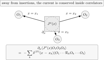
For $\mathcal O=\Phi_1(x_1)\Phi_2(x_2)$, define $I_R=\int_{\partial R}d\Sigma_\mu\langle J_\mu\mathcal O\rangle$. Region $A$ contains no insertion, so $I_A=0$; region $B$ contains only $x_1$, so $I_B=-\langle(R_1\Phi_1)\Phi_2\rangle$. The boundaries avoid the insertions, and the stated Ward hypotheses apply. Arrows show outward surface normals, not a current-flow pattern. The Euclidean section is schematic.

As a useful check, integrate the Ward identity over a region $R$. Gauss’s theorem gives

$$\int_R d^D x\,\partial_\mu\langle J_\mu(x)\mathcal O\rangle =\int_{\partial R} d\Sigma_\mu\,\langle J_\mu(x)\mathcal O\rangle.$$

If the boundary term vanishes and $R$ contains all insertions, then

$$\sum_{k=1}^n\langle\Phi_1\cdots R_k\Phi_k\cdots\Phi_n\rangle=0.$$

For a $U(1)$ correlator of charged fields, this becomes the charge-selection rule

$$\left(\sum_{k=1}^n e_k\right) \langle\Phi_1(x_1)\cdots\Phi_n(x_n)\rangle=0.$$

Thus a correlator in an invariant vacuum with no boundary flux can be nonzero only if the total charge is zero. A symmetry-breaking state or symmetry-breaking boundary condition removes this selection-rule premise; it need not be a state of nonzero total charge.

Momentum-space Ward identities

Ward identities are especially powerful in momentum space. With Euclidean momenta, define the full Fourier distribution

$$G_\mu(q;p_1,\ldots,p_n) =\int d^D x\prod_k d^D x_k\, e^{+iq\cdot x+i\sum_k p_k\cdot x_k} \langle J_\mu(x)\Phi_1(x_1)\cdots\Phi_n(x_n)\rangle.$$

This is the site-wide forward Fourier convention, so integration by parts gives $\partial_\mu\mapsto-iq_\mu$. Fourier transforming the position-space Ward identity therefore gives

$$\boxed{ q_\mu G_\mu(q;p_1,\ldots,p_n) =+\sum_{k=1}^n e_k\, G(p_1,\ldots,p_k+q,\ldots,p_n) }$$

for $U(1)$ fields, after the common factor of $i$ has been canceled. A source using the opposite phase is translated by reversing every momentum, $G_{\rm site}(q,p_k)=G_{-}( -q,-p_k)$; it then returns to the displayed formula. Changing the generator convention also changes the displayed charge sign. The invariant content is that contracting the current momentum is equivalent to inserting the symmetry generator on each charged leg.

The momentum-space figure follows one term of this identity: a position-space contact sets the current position equal to an insertion position, so their Fourier momenta add on that leg.

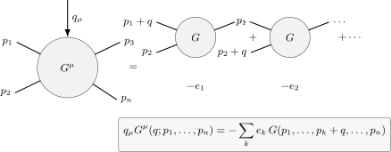
The two-point example uses incoming labels $-p-q$ and $p$ on fields of charges $+e$ and $-e$. A contact shifts exactly one label by $q$; the underline marks that change. After stripping the common translation delta, the contraction is $q_\mu G_\mu=e[G(p)-G(p+q)]$. Arrows denote Fourier momentum labels of correlators, not physical charge flow. The diagram is schematic; the amputation below fixes the proper-vertex identity.

For a charged scalar and its conjugate, choose the incoming Fourier labels $p_1=-p-q$ on $\phi$ and $p_2=p$ on $\phi^*$. Strip the common translation delta $(2\pi)^D\delta^{(D)}(q+p_1+p_2)$ from the three-point function and write the resulting current kernel as $G_\mu(p+q,p)$. For the rotationally invariant two-point kernel $G(p)$, the two opposite charges then give

$$q_\mu G_\mu(p+q,p)=e\,[G(p)-G(p+q)].$$

Where the full scalar propagators are invertible, define the amputated current vertex by

$$G_\mu(p+q,p)=G(p+q)\Gamma_\mu(p+q,p)G(p).$$

Then the Ward identity becomes

$$\boxed{ q_\mu\Gamma_\mu(p+q,p) =e\left[G^{-1}(p+q)-G^{-1}(p)\right]. }$$

This formula is one of the cleanest expressions of symmetry in perturbative QFT. It says that the longitudinal part of the current vertex is not independent dynamical data; it is fixed by the inverse propagator.

If the vertex has a direction-independent regular limit at $q=0$ and $G^{-1}$ is differentiable, expansion for arbitrary small $q$ gives

$$\Gamma_\mu(p,p)=e\,{\partial G^{-1}(p)\over\partial p_\mu},$$

in the Euclidean convention just defined. For a free scalar, $G^{-1}(p)=p_E^2+m^2$ and $\Gamma_\mu=e(2p+q)_\mu$ satisfy the finite-$q$ identity directly. A singular or direction-dependent soft vertex does not justify the limiting formula. In QED the corresponding matched Ward identity relates the vertex and fermion wavefunction renormalization factors; the renormalized charge also involves the photon normalization.

The first Goldstone pole

Ward identities also know about spontaneous symmetry breaking. Suppose a continuous symmetry acts nontrivially on an operator $\Phi$, and the vacuum expectation value is nonzero:

$$\langle\Phi\rangle=v\ne0.$$

Apply the Ward identity to the correlator $\langle J_\mu(x)\Phi(0)\rangle$. If

$$\delta\Phi=i e\alpha\Phi,$$

then

$$\partial_\mu\langle J_\mu(x)\Phi(0)\rangle =-i e v\,\delta^{(D)}(x).$$

Fourier transforming gives

$$q_\mu C_\mu(q)=ev, \qquad C_\mu(q)=\int d^D x\,e^{+iq\cdot x}\langle J_\mu(x)\Phi(0)\rangle.$$

Assume $ev\ne0$. If $C_\mu(q)$ were regular at $q=0$, the left side would vanish as $q\to0$, contradicting this identity. Its longitudinal projection is therefore

$$C_\mu^{\parallel}(q)=ev\,\frac{q_\mu}{q_E^2}, \qquad q_E^2=\sum_\mu q_\mu^2>0.$$

Regular transverse terms may also be present, but they cannot saturate the nonzero divergence.

Under the relativistic vacuum and positive spectral assumptions stated below, the massless longitudinal contribution has the Goldstone interpretation. The spectral step combines Lorentz covariance, locality, current conservation and a nonzero symmetry variation; see Weinberg 1995, Vol. II, § 19.2, pp. 169–172. A Euclidean projection formula alone is not a proof of all the hypotheses of a Lorentzian particle theorem.

The figure compares the regularity assumption with the nonzero divergence. Its upper plot uses the scalar longitudinal coefficient $F_L=ev/q_E^2$: for a reference momentum scale $\mu>0$, set $s=q_E^2/\mu^2$ and $f=\mu^2F_L/(ev)$. The pole gives $f=1/s$, while a regular control has $f=1$. The lower plot displays the corresponding contractions $sf=1$ and $sf=s\to0$. Only the pole maintains the required nonzero limit.

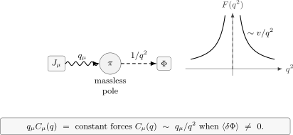
For $ev\ne0$, the Ward identity fixes $C_\mu^{\parallel}=evq_\mu/q_E^2$. The upper curves show exact dimensionless $f=1/s$ and the regular control $f=1$ on $0.1\le s\le1$; the lower curves compare their contractions as $s\downarrow0$. The open circle marks the pole’s limiting contraction, not a value of $f$ at zero. Solid and dashed styles distinguish the pole and control. These are normalized Euclidean functions, not a Lorentzian two-sided pole prescription. The next lesson supplies the further spectral interpretation.

Once the current Ward identity is established, this singularity argument does not require weak coupling or a classical potential. Its use of a noninvariant vacuum is consequential: the infinite-volume limit and state selection precede removal of an infinitesimal symmetry-breaking source. A finite symmetric integral does not itself select that state. The action-based derivation above is one way of obtaining the identity; an operator derivation can start from the same local current relation.

Scope of the pole argument

The symmetry here is a genuine continuous global internal symmetry, with a well-defined anomaly-free local current. Its selected infinite-volume vacuum is invariant under translations and Lorentz transformations, with locality and a positive-norm, positive-energy spectral representation. The nonzero variation is a limit of local current commutators; the proof need not assume a normalizable vector obtained by applying an unsmeared global charge to the vacuum. In $1+1$ dimensions, the usual local relativistic and tempered-distribution assumptions prevent this continuously broken vacuum, as proved in Coleman 1973, pp. 259–264 (PDF). The conditional Ward algebra remains correct, but its premise $ev\ne0$ is then unavailable. This obstruction does not exclude every massless state.

Summary

The Lorentzian commutator expectation of two local fields is the difference between two Wightman boundary values. For a conformal power law, this difference is a branch-cut discontinuity. It vanishes in the spacelike region because there the two boundary values coincide. On the light cone, and sometimes inside it, this discontinuity supplies the spectral function from which retarded and advanced response are built.

Current conservation has an equally local interpretation. A current is obtained by promoting a global symmetry parameter to $\alpha(x)$ and reading off the coefficient of $\partial_\mu\alpha$. Inside correlation functions, the divergence of this current vanishes away from operator insertions and produces contact terms at the insertions. These contact terms are Ward identities.

In momentum space, a Ward identity says that contracting a current insertion with its momentum is equivalent to acting with the symmetry generator on each external operator. If the chosen vacuum is not invariant, the same identity forces a massless pole: the first glimpse of Goldstone physics.

Common pitfalls

Confusing time ordering with response. The raw Feynman correlator $D_F$ is time ordered; the commutator expectation is the difference of two Wightman orderings. The former can be nonzero at spacelike separation. For a Hamiltonian source $H_{\rm ext}=-\int JO$, the causal response kernel is $\mathcal R=i\theta(t)\langle[O(x),O(0)]\rangle$, while the site’s $G_R=-i\theta(t)\langle[O(x),O(0)]\rangle=-\mathcal R$. These are the definitions in Lesson 17.

Dropping light-cone distributions. The off-cone formula with $\sin(\pi\Delta)$ can vanish at integer dimension while delta functions and their derivatives remain on the light cone. For noninteger dimension its global meaning also comes from the original boundary distribution.

Omitting contact terms. The equation $\partial_\mu J_\mu=0$ holds away from insertions. Charged insertions contribute the specified delta-function terms.

Ignoring the regulator or Jacobian. A Ward identity follows from an admissible change of variables, with the measure and boundary conditions accounted for. A noninvariant measure adds an anomaly; a nonzero boundary flux cannot simply be discarded.

Exercises

Exercise 1: The timelike discontinuity

Let

$$W_+(t,\mathbf x)={C\over(\rho+i0\operatorname{sgn}t)^\Delta}, \qquad W_-(t,\mathbf x)={C\over(\rho-i0\operatorname{sgn}t)^\Delta}, \qquad \rho=\mathbf x^2-t^2.$$

For non-integer $\Delta$, compute $W_+-W_-$ for $\rho>0$ and for $\rho<0$.

Solution

For $\rho>0$, the two boundary values approach the positive real axis from opposite sides. Since $\rho^{-\Delta}$ has no branch cut there,

$$(\rho+i0)^{-\Delta}=(\rho-i0)^{-\Delta}=\rho^{-\Delta}.$$

Therefore

$$W_+-W_-=0 \qquad (\rho>0).$$

For $\rho<0$, write $\rho=-|\rho|$. If $t>0$, then

$$\rho+i0=|\rho|e^{i\pi}, \qquad \rho-i0=|\rho|e^{-i\pi},$$

so

$$W_+-W_- =C|\rho|^{-\Delta}\left(e^{-i\pi\Delta}-e^{i\pi\Delta}\right) =-2iC\sin(\pi\Delta)|\rho|^{-\Delta}.$$

If $t<0$, the boundary prescriptions are reversed, so the result changes sign. Thus

$$W_+-W_- =-2iC\sin(\pi\Delta)\operatorname{sgn}t\,{\theta(-\rho)\over(-\rho)^\Delta}.$$

Since $-\rho=t^2-\mathbf x^2$, this is

$$W_+-W_- =-2iC\sin(\pi\Delta)\operatorname{sgn}t\, {\theta(t^2-\mathbf x^2)\over(t^2-\mathbf x^2)^\Delta}.$$

Exercise 2: Integer dimension and light-cone support

Use the distribution identity

$${1\over x+i0}-{1\over x-i0}=-2\pi i\delta(x)$$

to compute the commutator discontinuity for $\Delta=1$.

Solution

For $\Delta=1$,

$$W_+-W_-=C\left[{1\over\rho+i0\operatorname{sgn}t}-{1\over\rho-i0\operatorname{sgn}t}\right].$$

If $t>0$, this is

$$C\left({1\over\rho+i0}-{1\over\rho-i0}\right) =-2\pi iC\delta(\rho).$$

If $t<0$, the $i0$ prescriptions are reversed, giving the opposite sign. Hence

$$W_+-W_-=-2\pi iC\operatorname{sgn}t\,\delta(\rho).$$

Since $\rho=\mathbf x^2-t^2$, this distribution is supported on the light cone. This is the light-cone version of the massless free-field commutator.

Exercise 3: Deriving the current Ward identity

Derive the Ward identity

$$\partial_\mu\langle J_\mu(x)\Phi_1(x_1)\cdots\Phi_n(x_n)\rangle =-\sum_{k=1}^n\delta^{(D)}(x-x_k) \langle\Phi_1\cdots R_k\Phi_k\cdots\Phi_n\rangle$$

from a local change of variables in the Euclidean path integral, assuming the invariant regulator/measure and compactly supported parameter used in the text.

Solution

Let

$$\mathcal O=\Phi_1(x_1)\cdots\Phi_n(x_n).$$

Perform the infinitesimal change of variables

$$\delta\Phi_k=\alpha(x)R_k\Phi_k.$$

Assume the measure is invariant. Then

$$0=\int D\Phi\,\delta(e^{-S}\mathcal O) =\langle\delta\mathcal O\rangle-\langle\mathcal O\delta S\rangle.$$

The localized symmetry variation of the action is

$$\delta S=\int d^D x\,J_\mu\partial_\mu\alpha =-\int d^D x\,\alpha\partial_\mu J_\mu.$$

The insertion varies as

$$\delta\mathcal O= \sum_{k=1}^n\alpha(x_k)\Phi_1\cdots R_k\Phi_k\cdots\Phi_n.$$

Write this as an integral over $x$:

$$\delta\mathcal O= \int d^D x\,\alpha(x) \sum_{k=1}^n\delta^{(D)}(x-x_k) \Phi_1\cdots R_k\Phi_k\cdots\Phi_n.$$

Substituting into $0=\langle\delta\mathcal O\rangle-\langle\mathcal O\delta S\rangle$ gives

$$0=\int d^D x\,\alpha(x)\left[ \sum_{k=1}^n\delta^{(D)}(x-x_k) \langle\Phi_1\cdots R_k\Phi_k\cdots\Phi_n\rangle +\partial_\mu\langle J_\mu(x)\mathcal O\rangle \right].$$

Since $\alpha(x)$ is arbitrary, the integrand must vanish. This gives the Ward identity.

Exercise 4: The charge-selection rule

Let $\phi$ have $U(1)$ charge $+1$ and $\phi^*$ charge $-1$. Use the Ward identity to show that

$$\langle\phi(x_1)\phi(x_2)\rangle=0$$

in a symmetry-invariant vacuum, assuming the integrated current has no boundary flux.

Solution

For the two-point function

$$\mathcal O=\phi(x_1)\phi(x_2),$$

both insertions have charge $+1$. The integrated Ward identity for a region containing both insertions and with no boundary flux gives

$$(e_1+e_2)\langle\phi(x_1)\phi(x_2)\rangle=0.$$

Here $e_1=e_2=1$, so

$$2\langle\phi(x_1)\phi(x_2)\rangle=0.$$

Thus

$$\langle\phi(x_1)\phi(x_2)\rangle=0.$$

By contrast, $\langle\phi(x_1)\phi^*(x_2)\rangle$ is not forbidden, because the total charge is $1-1=0$.

Exercise 5: The zero-momentum Ward–Takahashi vertex

Use the Euclidean momentum routing and stripped translation delta defined in the text. Assume that $G^{-1}$ is differentiable, the vertex has a regular direction-independent limit as $q\to0$, and the current three-point function is written as

$$G_\mu(p+q,p)=G(p+q)\Gamma_\mu(p+q,p)G(p).$$

Starting from the Ward–Takahashi identity

$$q_\mu\Gamma_\mu(p+q,p)=e\left[G^{-1}(p+q)-G^{-1}(p)\right],$$

show that the zero-momentum current vertex is

$$\Gamma_\mu(p,p)=e{\partial G^{-1}(p)\over\partial p_\mu}.$$

Solution

Expand the inverse propagator for small $q$:

$$G^{-1}(p+q)=G^{-1}(p)+q_\nu{\partial G^{-1}(p)\over\partial p_\nu}+o(|q|).$$

Then the Ward–Takahashi identity becomes

$$q_\mu\Gamma_\mu(p+q,p) =e q_\nu{\partial G^{-1}(p)\over\partial p_\nu}+o(|q|).$$

Assuming the vertex is regular as $q\to0$, set

$$\Gamma_\mu(p+q,p)=\Gamma_\mu(p,p)+o(1).$$

The leading terms give

$$q_\mu\Gamma_\mu(p,p) =e q_\mu{\partial G^{-1}(p)\over\partial p_\mu}.$$

Since this holds for arbitrary infinitesimal $q_\mu$,

$$\Gamma_\mu(p,p)=e{\partial G^{-1}(p)\over\partial p_\mu}.$$

Exercise 6: The Goldstone singularity

Suppose a continuous symmetry current satisfies

$$\partial_\mu\langle J_\mu(x)\Phi(0)\rangle=-v\delta^{(D)}(x), \qquad v\ne0.$$

Show that the Fourier transform $C_\mu(q)$ cannot be regular at $q=0$.

Solution

Define

$$C_\mu(q)=\int d^D x\,e^{+iq\cdot x}\langle J_\mu(x)\Phi(0)\rangle.$$

The forward transform sends the derivative to $-iq_\mu$. Fourier transforming the assumed identity gives

$$q_\mu C_\mu(q)=-iv.$$

If $C_\mu(q)$ were regular at $q=0$, then $q_\mu C_\mu(q)$ would vanish as $q\to0$. This contradicts the nonzero right-hand side. Therefore $C_\mu(q)$ must be singular.

Rotational invariance implies that the singular longitudinal part has the form

$$C_\mu^{\parallel}(q)=-iv\,\frac{q_\mu}{q_E^2}, \qquad q_E^2>0.$$

Terms transverse to $q_\mu$ cannot saturate the nonzero divergence. The factor $-i$ follows from this exercise’s assumed contact $-v\delta$; the body’s different contact $-iev\delta$ instead gives $ev$. The Goldstone interpretation of the longitudinal singularity requires the vacuum and spectral hypotheses stated in the text.

References

• Coleman, Sidney. “There Are No Goldstone Bosons in Two Dimensions.” Communications in Mathematical Physics 31, no. 4 (1973): 259–264. Journal record. Open PDF.
• Di Francesco, Philippe, Pierre Mathieu, and David Sénéchal. Conformal Field Theory. Graduate Texts in Contemporary Physics. Springer, 1997. DOI.
• Gillioz, Marc. Conformal Field Theory for Particle Physicists: From QFT Axioms to the Modern Conformal Bootstrap. SpringerBriefs in Physics. Springer, 2023. DOI. Open PDF, arXiv:2207.09474v3, 3 May 2023. Locators above refer to the preprint’s printed page labels.
• Schwartz, Matthew D. Quantum Field Theory and the Standard Model. Cambridge University Press, 2014. DOI.
• Weinberg, Steven. The Quantum Theory of Fields, Volume II: Modern Applications. Cambridge University Press, 1995. DOI. Locators use the printed page labels of the consulted 2012 printing.