

Wick Theorem and n-Point Functions
The Feynman propagator is the two-point function of a free quantum field. The next question is what happens when more than two fields are inserted. In perturbation theory this is not a small technical issue: the Dyson expansion produces time-ordered products of many fields, and every term must be reduced to objects we know how to compute.
For a free field, the answer is exceptionally rigid. Once the two-point function is known, every vacuum time-ordered -point function is fixed. Odd-point functions vanish, and even-point functions are sums over all possible pairings of insertions. This is Wick theorem. It is the algebraic reason Feynman diagrams exist: a line is a two-point function, and a diagram is a bookkeeping device for a pattern of pairings.
The theorem is sometimes presented as a combinatorial trick. A better way to view it is this: a free field is a Gaussian quantum variable. Gaussian variables have no independent higher cumulants. Their higher moments are built entirely out of their two-point covariance. Wick theorem is the operator version of that Gaussian fact, with time ordering and the Feynman boundary condition built in.
Wick pairing formula
Section titled “Wick pairing formula”For a free real scalar field, Wick theorem says
while all odd vacuum correlators vanish. Here means , and a “complete pairing” means that every insertion appears in exactly one pair.
This boxed formula is the destination of the page. The rest of the derivation explains why the contraction is the Feynman propagator, why no other higher connected data appear in a free theory, and where the contact terms come from when the equation of motion acts on a time-ordered product.
Time ordering beyond two insertions
Section titled “Time ordering beyond two insertions”For two fields,
For three or more operators the definition is the same, but the notation becomes heavier. The time-ordering symbol rearranges operators so that later times stand to the left:
with analogous formulas in the other time-ordering regions. For bosonic operators there is no sign from the rearrangement. For fermionic operators each exchange contributes a minus sign; that will become important later.
The time-ordered vacuum expectation value is not merely a real-time object. The same expression can be understood by slightly complexifying the times. If
and is the latest operator in
then inserting energy eigenstates immediately to the right of gives terms of the form
These are positive-frequency contributions. To damp them at large positive time one sends the latest time slightly below the real axis:
Similarly, if is the earliest time, then
which is a negative-frequency contribution. It is damped by placing the earliest time slightly above the real axis:
This is the same Feynman boundary condition encoded by the prescription. In words: negative-frequency pieces are selected toward the past, while positive-frequency pieces are selected toward the future.
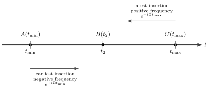
In a time-ordered vacuum matrix element, the latest insertion contributes phases , while the earliest insertion contributes phases . This is the time-domain form of the Feynman boundary condition.
Wick theorem now asks how this two-point object controls all higher products in a free theory.
Normal ordering and contractions
Section titled “Normal ordering and contractions”Split the oscillator into annihilation and creation parts,
Here the subscripts are bookkeeping for annihilation and creation parts. The term lowers the oscillator occupation number, while the term raises it. They are not charge labels and should not be confused with the charge labels used later for complex fields.
The notation is chosen so that annihilates the vacuum on the right and annihilates the vacuum on the left:
A normal-ordered product, written with colons, places all creation operators to the left of all annihilation operators:
Consequently, every vacuum expectation value of a nontrivial normal-ordered product vanishes:
The contraction of two fields is the difference between their time-ordered product and their normal-ordered product:
For a free oscillator this contraction is a c-number and equals the Feynman two-point function:
Indeed, if , then
If , the same argument gives the other time ordering. Together,
This is the same function obtained from the pole prescription. The point is that the contraction is not a new object; it is the Feynman propagator in operator clothing.
Two cautions are worth keeping in mind. First, normal ordering is defined relative to the chosen free vacuum and free oscillator split; changing the vacuum changes what “normal” means. Second, fields at the same spacetime point are operator-valued distributions, not ordinary functions. Wick theorem is safest when the insertions are kept at distinct points or smeared with test functions; coincident limits are where ultraviolet divergences enter.
Wick theorem
Section titled “Wick theorem”Wick theorem says that a time-ordered product of free fields equals the sum of all normal-ordered products obtained by contracting zero, one, two, and more disjoint pairs of fields:
where abbreviates and no field can be used in more than one contraction.
Taking the vacuum expectation value kills every remaining normal-ordered factor. Therefore the free time-ordered -point function is especially simple. Define
Then
A pairing is a partition of the labels into unordered pairs. The labels stay attached to the insertions throughout the calculation; Wick theorem is not saying that the points are indistinguishable. Time ordering is already contained inside each , so the pairing sum is over labels, not over time-ordering regions.
The number of pairings is
The denominator has a clear meaning: removes the order inside each pair, and removes the order of the pairs themselves.
For actual calculations, it helps to separate the algorithm from the formula:
- label the fields before doing any algebra;
- list complete pairings of the labels;
- replace each pair by or ;
- multiply within each pairing and sum over pairings.
Do not time-order the labels by hand after this step. The propagator attached to a pair is already the time-ordered two-point function.
The first nontrivial example is the four-point function:
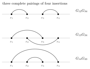
The free four-point function has three Wick pairings. The labels are not assumed to be time ordered; the time ordering is already contained in each propagator .
For six fields there are fifteen terms:
where the dots stand for all distinct pairings of the six labels. Listing them by hand is already unpleasant; drawing lines is better. This is the first taste of why diagrams are so efficient.
Proof by induction
Section titled “Proof by induction”The proof is almost the same as the proof of Gaussian moment factorization. For clarity, assume first that the times are ordered,
Then the vacuum correlator is
Write . Because , only the annihilation part contributes. Move to the right through . Each time it passes a field , it produces the c-number commutator
After the last commutation, the term with all the way on the right vanishes because . What remains is the exact recursion
where and the hat means that the argument is omitted. The recursion pairs label with exactly one of the other labels, then applies the same step to the remaining insertions. It therefore generates every complete pairing exactly once. If is odd, the recursion eventually reaches .
This proves the vacuum-correlator form of Wick theorem. The full operator identity stated above follows by the same commutation procedure before taking the vacuum expectation value: one must retain both the terms in which is contracted and all normal-ordered terms in which it remains uncontracted.
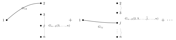
A recursive view of Wick theorem. Pair the first insertion with one of the remaining fields, remove both, and repeat. This generates each pairing exactly once.
For arbitrary real times, first divide the product into time-ordering regions and apply the ordered proof in each region. The result can be written uniformly because itself already knows which of and is later.
The same proof works for a free scalar field because each momentum mode is an oscillator. The only replacement is
Therefore
and all odd correlators vanish.
Contact-term recursion
Section titled “Contact-term recursion”The free field satisfies its equation of motion as an operator-valued distribution. Applying the wave operator to the complete time-ordered correlator also differentiates the ordering step functions and produces contact terms. This differs from inserting the vanishing free equation-of-motion operator inside ordinary time ordering. See Schwartz 2014, § 14.7.1, pp. 273–274; § 14.7.2, p. 275.
To obtain a differential form of Wick factorization, apply the wave operator to the correlator in its first argument. Since
the Wick expansion immediately gives
For the oscillator this becomes
Each term comes from differentiating the propagator joining the first argument to one other argument; the unpaired arguments form the lower-point correlator. The canonical contact-term derivation obtains the same sign from the equal-time commutator. The figure shows this differential operation on a propagator within the Wick expansion.
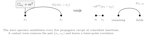
The wave operator acts on the full correlator in its first argument. In each Wick term it replaces the propagator joining that argument to another by , leaving a lower-point correlator.
For example, in the four-point function,
we get
The two-point function is the Feynman Green function with the displayed normalization. Higher-point functions obey the corresponding contact-term hierarchy; they are not themselves inverse kinetic kernels.
From oscillator modes to fields
Section titled “From oscillator modes to fields”The oscillator proof is not a toy calculation that later gets discarded. A free field is a continuum of independent oscillators, one for each momentum mode. Wick theorem for the field follows because the vacuum is Gaussian in all those oscillator coordinates simultaneously.
A real scalar field can be expanded in the covariantly normalized form
where . The field is therefore an infinite collection of oscillators. Wick theorem follows mode by mode, while the contraction becomes the spacetime propagator
The theorem is powerful because it separates two problems. The free theory supplies propagators. The interaction supplies insertions from the Dyson expansion. Perturbation theory is then the systematic pairing of free fields produced by those insertions.
This explains why the next step in the course is diagrammatic. A Wick pairing is a line. A product of pairings is a graph. Symmetry factors count how many algebraic pairings produce the same graph.
Summary
Section titled “Summary”Wick theorem is the central computational statement about free quantum fields. It says that every free vacuum time-ordered correlator is determined by the two-point function. Odd correlators vanish. Even correlators are sums over all pairings,
The theorem is the operator version of Gaussian moment factorization. Its physical content is that a free theory has no independent connected interactions: all higher correlations are built by propagating pairs of quanta between insertions.
The contact-term equation
is the differential form of the same statement. The complete time-ordered correlator obeys the homogeneous wave equation away from the contact support, while differentiating its time ordering produces the displayed delta-function sources. The underlying free operator equation remains exact. This is the bridge from Green functions to Feynman diagrams.
Common pitfalls
Section titled “Common pitfalls”The contraction is not an arbitrary line drawn between two fields. For the vacuum time-ordered theory it is exactly the Feynman propagator. Changing the boundary condition changes the contraction.
Normal ordering is not the same as time ordering. Normal ordering rearranges creation and annihilation operators; time ordering rearranges operators according to time. Wick theorem is useful precisely because it relates the two.
Do not forget the disconnected terms. In a free theory the four-point function is not zero, but it is disconnected:
A zero connected four-point function does not mean a zero four-point function.
For fermions, the same theorem holds with signs. Every interchange of fermionic fields contributes a minus sign. The scalar formulas on this page are the bosonic version.
A final overcounting check: for labeled insertions there is no additional numerical factor multiplying a Wick pairing. The coefficient is for each pairing. Symmetry factors appear later only after many labeled contractions are represented by the same unlabeled Feynman diagram.
Exercises
Section titled “Exercises”Exercise 1: Counting pairings
Section titled “Exercise 1: Counting pairings”Show that the number of pairings of labeled points is
Solution
Start with labeled points. If we order all labels in a sequence, there are possible sequences. Turn a sequence into pairs by grouping adjacent entries:
This overcounts each pairing. First, each pair can be written in two orders, giving a factor . Second, the pairs themselves can be permuted, giving a factor . Hence
Equivalently, choose a partner for point in ways, then a partner for the smallest remaining label in ways, and so on:
Exercise 2: Six-point Wick expansion
Section titled “Exercise 2: Six-point Wick expansion”Use Wick theorem to compute the free six-point function
in the partially organized form where is paired first.
Solution
Pair with one of the other five times. For each choice, Wick theorem gives the propagator for that pair times the four-point function of the remaining fields:
There are terms, as expected from
Exercise 3: Contact terms in a four-point function
Section titled “Exercise 3: Contact terms in a four-point function”Let
Using , prove the contact-term identity for .
Solution
Act with . Only propagators containing are differentiated. Therefore
Using
we obtain
which is the case of the general recursion formula.
Exercise 4: Complex scalar pairings
Section titled “Exercise 4: Complex scalar pairings”For a complex free scalar field with nonzero contractions
compute
Solution
Only contractions between a and a are nonzero. Therefore there are two pairings:
and
Thus
This is the complex-field version of Wick factorization, with charge conservation built into the allowed contractions.
References
Section titled “References”- Schwartz, Matthew D. Quantum Field Theory and the Standard Model. Cambridge: Cambridge University Press, 2014. DOI.
Further reading
Section titled “Further reading”- Sidney Coleman, Lectures of Sidney Coleman on Quantum Field Theory, Chapter 8, for Wick theorem and the transition from Wick diagrams to perturbation theory.
- Mark Srednicki, Quantum Field Theory, Sections 8–10, for the path-integral derivation of free-field correlators and Feynman rules.
- Steven Weinberg, The Quantum Theory of Fields, Volume I, Sections 6.1–6.2, for Wick pairings, coordinate-space rules, and propagators in perturbative QFT.
- Michael E. Peskin and Daniel V. Schroeder, An Introduction to Quantum Field Theory, Chapter 4, for the standard perturbative use of Wick theorem in scalar field theory.
Original QFT.org content:CC BY 4.0, unless an item supplies different terms. Third-party material retains its own terms.