The Dirac equation by itself is a relativistic wave equation for spinors. A quantum field theory of spin-21 particles requires one more step: the spinor solution must become an operator-valued field. The modes of this field create and destroy particles and antiparticles, and the algebra of those modes must be fermionic.
This is the first place in the course where the sign rules of fermions become unavoidable. The scalar field was quantized by commutators. The Dirac field is quantized by anticommutators. That change is not cosmetic: it is what turns the negative-frequency solutions of the Dirac equation into positive-energy antiparticles, enforces the Pauli principle, and produces the minus signs in fermion loops and fermionic Wick contractions.
The practical goal is to connect three statements that are often learned separately: the vs(p)e+ip⋅x branch creates antiparticles, the equal-time anticommutator is local, and the momentum-space propagator has numerator γ⋅p+m. They are not separate miracles; they are the same free-field construction viewed from three angles.
Required background.Dirac equation and spinor solutions supplies the plane-wave equations, Dirac adjoint, spinor normalization, and completeness relations used below.
The label s=1,2 denotes the two spin states. In a relativistic quantum field theory both families must appear. If one tried to keep only the positive-frequency u modes, the field anticommutator would fail to have the locality properties required by relativity. The v modes are not optional bookkeeping; they are the antiparticle sector of the field.
Here bs†(p) creates a particle, bs(p) annihilates a particle, ds†(p) creates an antiparticle, and ds(p) annihilates an antiparticle. This page uses the common canonical oscillator normalization, in which the factors 1/2Ep sit in the field expansion and the mode anticommutators contain no 2Ep.
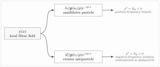
The Dirac field contains a particle-annihilation term bs(p)us(p)e−ip⋅x and an antiparticle-creation term ds†(p)vs(p)e+ip⋅x. The two branches are tied together by Lorentz covariance and by locality.
The vacuum obeys
bs(p)∣0⟩=0,ds(p)∣0⟩=0.
With the oscillator normalization above, the simple Fock states are
They have noncovariant delta-function normalization. When these states are used in LSZ or invariant phase space formulas, replace them by the covariant states 2Epbs†∣0⟩ and 2Epds†∣0⟩. Keeping this dictionary explicit prevents the most common factor-of-2E mistake in spinor amplitudes.
The conserved number current is
jμ=ψˉγμψ.
For a field of charge q, the normal-ordered charge is
Q=qs∑∫(2π)3d3p(bs†(p)bs(p)−ds†(p)ds(p)).
Thus the d† excitation has the opposite charge. For the electron field one usually takes q=−e, so the b† excitation is an electron and the d† excitation is a positron.
The momentum conjugate to ψα† vanishes. Thus the first-order Dirac Lagrangian is a constrained system: π−iψ†≃0 and π†≃0 are second-class constraints. A full Dirac-bracket analysis leads to the equal-time relation below once the classical graded bracket is promoted to an operator anticommutator. Relativistic locality and a Hamiltonian bounded below select this fermionic quantization; first-order time evolution alone is not a proof of spin–statistics.
{ψα(t,x),ψβ†(t,y)}=δαβδ(3)(x−y),
with
{ψα(t,x),ψβ(t,y)}=0,{ψα†(t,x),ψβ†(t,y)}=0.
Equivalently, with the 1/2Ep mode expansion above, the mode operators satisfy
and all other anticommutators vanish. If one wants covariantly normalized one-particle states, define ∣p,s⟩cov=2Epbs†(p)∣0⟩ and similarly for antiparticles. Then
cov⟨p′,s′∣p,s⟩cov=(2π)32Epδ(3)(p−p′)δss′.
The Pauli principle is immediate:
{bs†(p),bs†(p)}=2bs†(p)bs†(p)=0,
so one cannot create two identical fermions in exactly the same quantum state.
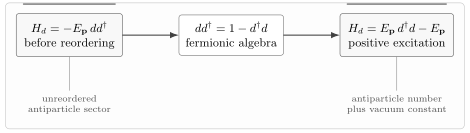
There is also a deeper energy argument. To manipulate coincident modes, first use a periodic box of volume V and a finite momentum set Λ. The discrete oscillators have unit CAR, {dps,dqr†}=δpqδsr, rather than a Dirac delta. Before normal ordering, the free Hamiltonian is
Here Evac=−∑p∈Λ,sEp is finite before the regulator is removed. Normal ordering subtracts the selected free-vacuum energy. Both particles and antiparticles then carry positive excitation energy. If the d modes obeyed ordinary commutators, the sign would not flip in this way, and the theory would contain negative-energy excitations. The continuum expression restores the volume factor in the vacuum constant Schwartz 2014, § 12.5.2, pp. 217–218, Eqs. (12.65)–(12.68); the canonical Dirac Hamiltonian treatment gives the finite-box construction.
For one unit-normalized discrete mode, dd†=1−d†d turns the d sector into a positive-energy antiparticle excitation plus its negative vacuum constant. The schematic figure shows the finite-mode algebra, not a replacement of a continuum delta by one.
This is the free-field manifestation of the spin–statistics connection. A full spin–statistics theorem is deeper, but already here locality, positivity of energy, and the exclusion principle are all pointing to the same algebra.
In the second term change integration variable p↦−p. The spatial part of γ⋅p=γ0Ep−γ⋅p changes sign, while the energy and mass terms do not. The two terms combine to
The antiparticle contribution is essential in this cancellation. Without the v modes, the equal-time algebra would not collapse to the local delta function.
The same statement extends away from equal time. Define the scalar Pauli–Jordan distribution
Δ(z)=∫(2π)32Epd3p(e−ip⋅z−e+ip⋅z),p0=Ep.
Then the mode expansion gives
{ψα(x),ψˉβ(y)}=(iγμ∂xμ+m)αβΔ(x−y).
This local Δ is the raw scalar commutator kernel; in the convention [ϕ(x),ϕ(y)]=iΔPJ(x−y) it equals iΔPJ. Because this distribution and its derivatives vanish on the open spacelike region, the Dirac field satisfies fermionic microcausality. Both the u and v sectors are needed for this cancellation.
The minus sign is the whole story. It is the same sign that appears when exchanging two fermionic creation operators, and it will become the sign attached to closed fermion loops in perturbation theory.
The Feynman propagator is
SF,αβ(x−y)=⟨0∣T{ψα(x)ψˉβ(y)}∣0⟩.
Some books instead define iSF to be the time-ordered expectation value. Here SF itself is the expectation value, so its Fourier transform and the internal-line factor are
These two pieces combine into the compact four-dimensional expression
SF(x−y)=∫(2π)4d4pp2−m2+iϵi(γ⋅p+m)e−ip⋅(x−y).
In momentum space,
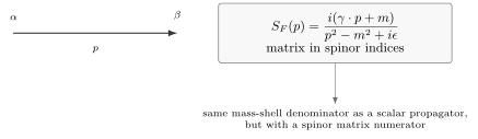
SF(p)=p2−m2+iϵi(γ⋅p+m).
One often writes this suggestively as i/(γ⋅p−m) with the Feynman prescription understood. The precise formula is the fraction above: the inverse of the Dirac operator is obtained by multiplying by γ⋅p+m, while the iϵ prescription belongs to the scalar denominator p2−m2+iϵ. The pole locations are the same as for a scalar particle; the numerator is now a spinor matrix.
A fermion propagator is a matrix in spinor indices. In momentum space the line carries SF(p)=i(γ⋅p+m)/(p2−m2+iϵ). The arrow tracks fermion-number flow, not necessarily momentum flow.
The propagator is the Green function of the Dirac operator:
(iγμ∂xμ−m)SF(x−y)=iδ(4)(x−y)14.
This sign matches the scalar convention DF(p)=i/(p2−m2+iϵ) because SF(p)=(γ⋅p+m)DF(p) as a matrix-valued distribution.
This is the spinor analogue of the scalar equation
(∂x2+m2)GF(x−y)=−iδ(4)(x−y).
For the Dirac field the differential operator is first order, but the pole structure is still the mass-shell pole p2=m2.
The source of the delta function in the Green-function equation is the same as in the scalar case: differentiating the step functions in the time-ordered product creates a contact term. For fermions,
When iγ0∂x0 acts on the step functions, it produces
iγ0δ(x0−y0)⟨0∣{ψ(x),ψˉ(y)}∣0⟩.
Using the equal-time anticommutator,
{ψα(t,x),ψˉβ(t,y)}=(γ0)αβδ(3)(x−y),
this becomes precisely the four-dimensional contact term
iδ(4)(x−y)δαβ.
Away from x=y, the two Wightman functions solve the homogeneous Dirac equation, so only the contact term remains. This is why the propagator is the inverse of the Dirac operator as a distribution, not as an ordinary function.
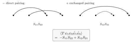
The direct pairing appears with a plus sign and the exchanged pairing with a minus sign. This alternating order is the determinant of the matrix of contractions SF,αiβj(xi−yj). If the two ψ fields are instead grouped before the two ψˉ fields, one odd interchange changes the overall sign:
⟨0∣T{ψ1ψ2ψˉ1ψˉ2}∣0⟩=−S11S22+S12S21.
Thus the order written on the page is part of the formula; “the determinant sign” is not independent of that order.
A useful way to remember the rule is this:
fermionic Wick sum=pairings∑(−1)Ppairs∏SF,
where P is the parity of the permutation required to move the paired fermionic operators next to one another.
For the grouped order ψ1ψ2ψˉ1ψˉ2, the direct pairing has a minus sign and the exchanged pairing has a plus sign. Reordering the fields to ψ1ψˉ1ψ2ψˉ2 reverses the overall sign and yields the familiar determinant S11S22−S12S21.
For a Majorana field the distinction between particle and antiparticle is absent, and contractions between two Majorana fields are possible after inserting the charge-conjugation matrix. The sign principle is unchanged: every exchange of fermionic operators contributes a minus sign.
The scalar propagator carried one number per momentum. The Dirac propagator carries a 4×4 matrix because it propagates spinor information. The matrix multiplication order is fixed by the orientation of the fermion line; reversing it is not an innocent cosmetic change. An internal fermion line in a Feynman diagram therefore contributes
p2−m2+iϵi(γ⋅p+m),
with spinor indices contracted along the line. The arrow on the line is not decoration. It tells us how to multiply the matrices and how charge flows through the diagram.
A typical bilinear coupling to a scalar field has the form
Lint=−gϕψˉψ.
A chain of fermion propagators and vertices then gives a matrix product such as
uˉ(p′)[(−ig)SF(k1)(−ig)SF(k2)⋯(−ig)]u(p),
where the order of matrices is the order along the fermion line. This is one of the first practical differences between scalar and spinor perturbation theory: spinor diagrams carry matrix algebra as well as momentum integrals.
A second difference is the closed-loop sign. Relative to the analogous bosonic contraction, closing a chain of fermionic contractions leaves one odd cyclic reordering. Consequently each independent closed fermion loop contributes a factor
−1.
The loop also involves a trace over spinor indices. Thus a closed fermion loop usually produces an expression of the schematic form
−∫(2π)4d4ℓtr[SF(ℓ)Γ1SF(ℓ+k1)Γ2⋯],
where the Γi are the spinor matrices appearing in the vertices.
The quantized Dirac field is built from two kinds of ladder operators. The b† operators create particles, while the d† operators create antiparticles. Both appear in the same local spinor field.
The crucial new ingredient is the fermionic algebra. Equal-time anticommutators give a local delta function, enforce the exclusion principle, and convert the negative-frequency branch of the classical Dirac equation into positive-energy antiparticles. This is why the normal-ordered Hamiltonian contains
Ep(b†b+d†d)
rather than a negative-energy antiparticle sector.
The Dirac propagator is the inverse of the first-order operator iγμ∂μ−m:
SF(p)=p2−m2+iϵi(γ⋅p+m).
It has the same mass-shell denominator as the scalar propagator but a matrix numerator that carries spinor information. Fermionic time ordering introduces minus signs, and fermionic Wick contractions therefore have determinant-like signs rather than purely permanent-like bosonic signs.
A frequent mistake is to say that vs(p) is simply a negative-energy particle spinor. In the field operator, the vs(p)e+ip⋅x term multiplies ds†, so it creates a positive-energy antiparticle.
Another common mistake is to forget the minus sign in fermionic time ordering. Without it, the Dirac propagator would not be the correct inverse of the Dirac operator, and Wick’s theorem would give wrong relative signs.
It is also easy to confuse momentum flow with arrow flow. The arrow on a fermion line tracks fermion-number flow and spinor-index contraction. Momentum may be assigned along or against the arrow, as long as it is done consistently.
Do not mix the oscillator normalization used in the mode expansion with the covariant state normalization used in cross sections. The conversion factor is 2Ep per external one-particle state.
Finally, the expression
γ⋅p−mi
is only shorthand for a matrix inverse with the scalar Feynman pole prescription understood. The explicit propagator is
into a positive antiparticle Hamiltonian plus a constant.
Solution
Using
{ds(p),ds′†(q)}=(2π)3δss′δ(3)(p−q),
first replace the continuum by the same finite box and momentum set as in the Hamiltonian derivation. For each discrete mode,
dd†=1−d†d.
Therefore
Hd,Λ=−p∈Λ,s∑Ep(1−ds†(p)ds(p)).
Thus
Hd,Λ=p∈Λ,s∑Epds†(p)ds(p)+Evac,Λ,
where
Evac,Λ=−p∈Λ,s∑Ep.
At fixed UV cutoff, the large-volume limit gives
VEvac,Λ⟶−s∑∫Λ(2π)3d3pEp.
Thus the integral is an energy density, with mass dimension four; the total energy has the extra V=(2π)3δ(3)(0) in continuum notation. Removing the UV cutoff makes this free-vacuum constant divergent. Normal ordering leaves the positive excitation spectrum; it is not a calculation of gravitational vacuum energy.