

Scattering Amplitudes and Dyson Resummation
The previous pages taught us to read physics from singularities of Green functions: poles describe stable particles, cuts describe continua, and imaginary parts appear when intermediate states can go on shell. This page turns that analytic information into a scattering amplitude. The cleanest setting is nonrelativistic potential scattering, because it contains the same architecture as relativistic QFT but without spin, antiparticles, or complicated phase space.
The central idea is that a Green function contains two kinds of information. Its external propagators describe how free particles travel to and from the interaction region. Its middle part describes the actual scattering. To get the scattering amplitude, we amputate the external propagators and put the remaining object on shell. The result is the -matrix.
The same organization also explains Dyson resummation. Instead of summing every diagram from scratch, one isolates a kernel that cannot be separated by cutting a chosen propagator, and then sums repeated insertions of that kernel. For a one-particle propagator the kernel is the self-energy. For potential scattering the kernel is the potential, or more generally an irreducible scattering kernel.
The key distinction for this page is:
| Object | Off shell? | Contains external propagation? | Directly observable? |
|---|---|---|---|
| yes | yes | no | |
| yes | no | no | |
| no | no | yes, through and cross-sections |
The off-shell objects are essential for calculation, but the physical scattering amplitude is the on-shell amputated object.
Free propagation in a potential background
Section titled “Free propagation in a potential background”Assume is self-adjoint and admits the usual short-range incoming and outgoing scattering states. A real, smooth, rapidly decaying local potential is the concrete setting here. Interpret momentum eigenstates distributionally through wave packets, and take boundary values at positive energies away from thresholds and poles. The resolvent below selects the outgoing scattered wave; it does not by itself prove existence of the asymptotic limits. The in/out-state treatment explains what those limits require.
Consider a nonrelativistic field moving in a time-independent external potential . A convenient quadratic action is
The equation of motion is the Schrödinger equation
In the absence of , the time-ordered Green function is
The prescription says that a particle propagates forward in time. For , closing the contour in the lower half-plane gives
while for the contour encloses no pole. This is the nonrelativistic version of the causal boundary condition already used for the Feynman propagator.
The potential has momentum-space matrix element
Because the potential is time-independent, it conserves energy but not necessarily momentum. Each insertion of changes the spatial momentum by the amount carried by the background.
The Born series as a Green-function expansion
Section titled “The Born series as a Green-function expansion”The exact Green function in the potential background obeys the operator identity
Iterating it gives the Born series
In momentum space,
The first term is free propagation. The second term says that the particle propagates freely, scatters once, then propagates freely again. The third term has one intermediate momentum integral and two scatterings. Higher terms repeat the same pattern.
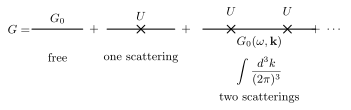
The Born series for the Green function in a background potential. Thin lines denote , crosses denote insertions of , and the intermediate momenta are integrated over. The external free propagators will be removed when extracting the scattering amplitude.
This expansion is the nonrelativistic ancestor of perturbation theory in QFT. The only difference is the meaning of the vertex. Here is a fixed external potential; in QFT, vertices come from interaction terms in the action and internal lines can represent all allowed virtual particles.
Amputated Green functions
Section titled “Amputated Green functions”It is inefficient to keep writing the external propagators. Define the amputated scattering kernel by
Then the Born series for is
Equivalently, satisfies the Lippmann–Schwinger equation
In momentum variables this means
The equation is not merely a mnemonic for perturbation theory. It is also a resummation: if the integral equation can be solved, it contains infinitely many potential insertions.

The amputated kernel satisfies . This is the potential-scattering version of the Dyson idea: isolate a kernel and sum its repeated insertions connected by free propagation.
The word “amputated” means exactly what it sounds like. The full connected Green function contains external factors and . Removing them leaves . This step is algebraic and can be done off shell.
The next step is physical: scattering states live on the mass shell, so the physical -matrix is the on-shell value
This formula is the simplest version of LSZ logic: amputate the external propagators and put the external particles on shell.
How energy conservation emerges
Section titled “How energy conservation emerges”The on-shell delta function arises from the long-time limit. Look at the connected part of the two-point Green function,
Fourier transform it over a long time interval. If is smooth near the external poles, the singular part is controlled by
For , the poles lie just below the real axis. Evaluating their residues gives a difference of two oscillatory exponentials divided by the energy difference:
Because has no overall factor of in our convention, its Fourier transform is times the evolution kernel. Thus the connected Schrödinger-picture evolution amplitude is . To obtain the interaction-picture -matrix between symmetric endpoints and , strip the free phases from both external states:
where the smooth kernel may be evaluated at the common energy in the distributional on-shell limit. Now
and therefore the transition part of the -matrix has the form
where is the on-shell amputated kernel. The explicit phase stripping is essential: the resolvent transform by itself is a Schrödinger-picture propagation amplitude, not yet the -matrix. After that step, the external propagator poles select the on-shell value of and supply the energy-conserving delta function.
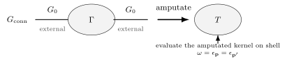
The connected Green function factorizes as . The scattering amplitude is obtained by removing the external propagators and evaluating the remaining kernel at .
Discontinuities and on-shell intermediate states
Section titled “Discontinuities and on-shell intermediate states”Suppose a contribution is built from two subkernels and joined by one free intermediate propagator. Before any on-shell limit, their composition is
The intermediate momentum is off shell in this ordinary product. It is placed on shell only when we take the discontinuity of the propagator. If and have no discontinuity in the channel under discussion, then
This is the one-particle version of a much broader principle: discontinuities factorize through the phase space of intermediate on-shell states. In relativistic QFT the one-particle measure becomes
and the delta functions impose full four-momentum conservation. The optical theorem and cutting rules are sophisticated versions of the same statement.
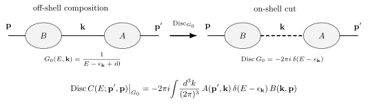
The ordinary composition contains an off-shell propagator. Its discontinuity replaces that propagator by , exposing the phase space of a real intermediate particle.
This is also where reducible and irreducible diagrams become useful language. A diagram is reducible with respect to a chosen propagator if cutting that propagator separates the diagram into two pieces. The repeated terms in the Born series are reducible in this sense. The potential is the irreducible kernel for the simple problem above. In an interacting QFT, the corresponding kernel is often a sum of many diagrams that are irreducible with respect to the relevant cut.
Dyson resummation as a general strategy
Section titled “Dyson resummation as a general strategy”The self-energy resummation from earlier pages had the form
This geometric series gives
Potential scattering has the parallel structure
and therefore
The exact same logic appears later in many forms:
The common lesson is that the object one should compute is rarely the full answer diagram by diagram. It is usually better to compute an irreducible building block and then let an integral equation perform the resummation.
Example: first Born approximation
Section titled “Example: first Born approximation”At leading order,
For elastic scattering, , and the momentum transfer is
With the normalization used here, the nonrelativistic scattering amplitude is related to the -matrix by
so
For a weak Gaussian potential
we have
Therefore the first Born cross-section is
Forward scattering is largest because the Fourier transform of a smooth potential is largest at small momentum transfer. A short-range potential gives a broad angular distribution; a long-range smooth potential strongly favors small angles.
Summary
Section titled “Summary”The scattering amplitude is the on-shell, amputated part of a Green function. In the nonrelativistic potential problem,
The external propagator poles provide the energy-conserving delta function in the -matrix, while the amputated kernel contains the real scattering dynamics.
The Born series is a perturbative expansion in the potential:
Written as
it becomes the Lippmann–Schwinger equation. This is the scattering version of Dyson resummation: isolate an irreducible kernel, then sum its repeated insertions. The same strategy organizes self-energies, scattering amplitudes, Bethe–Salpeter equations, and eventually the effective action.
Common pitfalls
Section titled “Common pitfalls”Confusing the Green function with the scattering amplitude. The full Green function includes external propagation before and after the collision. The scattering amplitude is the amputated, on-shell kernel.
Putting internal lines on shell too early. The internal line in the Lippmann–Schwinger equation is and is integrated over all . An on-shell delta function appears only when taking a discontinuity or an appropriate long-time/asymptotic projection.
Losing the prescription. The sign of decides whether the solution is outgoing or incoming. Scattering theory is not just algebraic inversion; it is inversion with a boundary condition.
Mixing normalization conventions. The relation between and changes if one uses box-normalized states or relativistic normalization. The invariant content is the -matrix element with its stated state normalization.
Calling every resummation “Dyson” without naming the kernel. A resummation becomes meaningful only after specifying what is irreducible. For the one-particle propagator it is the 1PI self-energy ; for potential scattering it is or a more general irreducible scattering kernel .
Forgetting that off-shell kernels are not observables. depends on how the calculation is organized. The on-shell -matrix, with the stated normalization, is what enters scattering probabilities.
Exercises
Section titled “Exercises”Exercise 1
Section titled “Exercise 1”Starting from the Born series
show that obeys both
and
Solution
Factor the Born series after the first :
The expression in parentheses is , so
Alternatively, factor the last :
Again the parenthesis is , giving
The two equations are equivalent for the same Born series. Written in momentum space, they differ in whether the potential next to the external final leg or the external initial leg is singled out.
Exercise 2
Section titled “Exercise 2”Use the distribution identity
to find the imaginary part of the second Born term
Specialize to forward scattering, , with , and take to be Hermitian.
Solution
Apply the identity with :
Therefore
The imaginary part is produced only by intermediate momenta satisfying the on-shell condition . Its negative sign is consistent with this page’s convention (and with ). This is the second-order, nonrelativistic shadow of the forward optical theorem and the cutting rule.
Exercise 3
Section titled “Exercise 3”For the Gaussian potential
compute the first Born approximation to using
Solution
The Fourier transform is
Using the standard Gaussian integral gives
For elastic scattering, . Hence
Therefore
The angular distribution narrows as grows, because a wider potential has a narrower Fourier transform.
Exercise 4
Section titled “Exercise 4”Consider a separable potential
where is real and is smooth and rapidly decaying in momentum space. This is a bounded, generally nonlocal rank-one potential; the operator Lippmann–Schwinger equation still applies. Use a positive energy at which the outgoing boundary value exists, and solve for away from its poles.
Solution
Use the ansatz
Substitute into
The right-hand side is
Thus
where
Solving,
and therefore
A pole occurs when . Depending on its location, this pole describes a bound state, a resonance, or an instability of the perturbative expansion.
References and further reading
Section titled “References and further reading”- B. A. Lippmann and J. Schwinger, “Variational Principles for Scattering Processes,” Physical Review 79 (1950), for the original integral-equation formulation of scattering states.
- Steven Weinberg, The Quantum Theory of Fields, vol. I, sections 3.1–3.6 and 10.3, for scattering states, the -matrix, perturbation theory, and pole extraction.
- Sidney Coleman, Lectures on Quantum Field Theory, chapters 7, 10–14, for perturbation theory, scattering, phase space, and the LSZ viewpoint.
- Mark Srednicki, Quantum Field Theory, sections 5, 10, and 13–14, for LSZ reduction, scattering amplitudes, and exact propagator structure.
- M. L. Goldberger and K. M. Watson, Collision Theory, for a classic systematic treatment of potential scattering, the -matrix, and the Lippmann–Schwinger equation.
Original QFT.org content:CC BY 4.0, unless an item supplies different terms. Third-party material retains its own terms.