OPE, Associativity, and Conformal Correlators

Conformal symmetry fixes scalar two- and three-point functions up to constants, while four-point functions retain dynamical information. The operator product expansion (OPE) organizes that information into exchanged operator families; requiring different pairings to give the same correlation function produces crossing symmetry. This lesson develops those statements for separated insertions in a unitary Euclidean CFT in $d\ge2$, with a conformally invariant vacuum, radial quantization and a discrete local operator spectrum.

The spectrum lists local primary operators and their dimensions, spins and symmetry representations. OPE coefficients specify how their products expand. Together with the spacetime dimension, symmetry algebra and two-point normalization, these data reconstruct local correlators through convergent OPEs and their continuation. They do not by themselves specify every possible defect or global completion. The Ising example below also shows why a normalized two-point function does not fix an operator’s sign.

Required background. Lesson 14 supplies connected conformal transformations, primary covariance and the scalar Ward identity used below.

Helpful background. Lesson 12 develops scaling operators and the Ising examples, while Lesson 13 explains how fixed-point correlators acquire homogeneous scaling laws.

Scalar two-point functions

Distances and active primary transformations

We work in Euclidean signature. We distinguish the displacement vector

$$x_{ij}^\mu=x_i^\mu-x_j^\mu$$

from its Euclidean length $x_{ij}=|x_i-x_j|$; thus $x_{ij}^2=(x_i-x_j)^2$. Scalar primaries $O_i$ have scaling dimensions $\Delta_i$. Under a conformal transformation $x'=f(x)$ with local length scale $\Omega(x)$,

$$O_i'(x')=\Omega(x)^{-\Delta_i}O_i(x).$$

The main argument uses the connected conformal group. The coordinate inversion $x'=x/x^2$ has $\Omega(x)=1/x^2$, but its action as a quantum symmetry requires a separate assumption.

For scalar primaries, translation and rotation invariance imply that a two-point function depends only on $x_{12}$. Scale covariance permits

$$\langle O_i(x_1)O_j(x_2)\rangle ={C_{ij}\over x_{12}^{\Delta_i+\Delta_j}}.$$

The special-conformal Ward identity from Lesson 14, with the second insertion at the origin, additionally requires

$$(\Delta_i-\Delta_j)x_\alpha \langle O_i(x)O_j(0)\rangle=0.$$

Thus the coefficient vanishes unless the dimensions agree. Writing the surviving coefficients as $g_{ij}$ gives

$$\boxed{ \langle O_i(x)O_j(0)\rangle ={g_{ij}\over |x|^{2\Delta_i}}, \qquad g_{ij}=0\quad \text{unless }\Delta_i=\Delta_j. }$$

After removing null states, reflection positivity gives a positive two-point form with the appropriate adjoint insertion. For the formulas below choose an orthonormal Hermitian scalar basis within each compatible symmetry sector,

$$g_{ij}=\delta_{ij}.$$

This is a basis choice. It fixes the magnitudes of field normalizations but still permits sign changes of Hermitian fields, or orthogonal rotations among degenerate fields; OPE coefficients transform with that choice. Complex charged fields instead pair with their adjoints.

Three-point functions

Translation and rotation invariance allow a scalar three-point function $G_3$ to depend on the three pair distances. Connected special-conformal covariance removes the remaining freedom. For $n$ scalar insertions its Ward identity is

$$\sum_{a=1}^n \left[2x_{a\alpha}x_a\cdot\partial_a -x_a^2\partial_{a\alpha}+2\Delta_a x_{a\alpha}\right]G_n=0.$$

An infinitesimal special-conformal map with parameter $b$ changes a pair distance by $\delta\log x_{ij}=b\cdot(x_i+x_j)$. Define $D_{ij}=x_{ij}\partial/\partial x_{ij}$. For three generic non-collinear points, the Ward identity and dilation covariance give

$$\begin{aligned} (D_{12}+D_{13})G_3&=-2\Delta_1G_3,\\ (D_{12}+D_{23})G_3&=-2\Delta_2G_3,\\ (D_{13}+D_{23})G_3&=-2\Delta_3G_3. \end{aligned}$$

To see why the coefficients separate, collect the Ward expression by $x_1$, $x_2$ and $x_3$. Their coefficient sum vanishes by dilation covariance; after translating $x_3$ to zero, the two remaining vectors are independent. Solving these first-order equations and extending to separated collinear configurations gives a product of powers,

$$\langle O_1(x_1)O_2(x_2)O_3(x_3)\rangle ={C_{123}\over x_{12}^{a}x_{23}^{b}x_{13}^{c}}.$$

Scale covariance requires

$$a+b+c=\Delta_1+\Delta_2+\Delta_3.$$

The three Ward equations require

$${a+c\over2}=\Delta_1, \qquad {a+b\over2}=\Delta_2, \qquad {b+c\over2}=\Delta_3.$$

Solving gives

$$a=\Delta_1+\Delta_2-\Delta_3,$$ $$b=\Delta_2+\Delta_3-\Delta_1,$$ $$c=\Delta_1+\Delta_3-\Delta_2.$$

Therefore

$$\boxed{ \langle O_1(x_1)O_2(x_2)O_3(x_3)\rangle ={C_{123}\over x_{12}^{\Delta_1+\Delta_2-\Delta_3} x_{23}^{\Delta_2+\Delta_3-\Delta_1} x_{13}^{\Delta_1+\Delta_3-\Delta_2}} .}$$

This proof needs no discrete inversion symmetry. Exercise 1 checks the same powers by inversion when that extra symmetry is present.

The constants $C_{123}$ are the first genuinely dynamical CFT data. Symmetries may force some of them to vanish. For example, in the Ising CFT the global spin-flip symmetry sends $\sigma\mapsto -\sigma$, so a correlator with an odd number of $\sigma$ insertions vanishes:

$$C_{\sigma\sigma\sigma}=0.$$

The three-point coefficient $C_{\sigma\sigma\varepsilon}$ is allowed and controls the first nontrivial term in the $\sigma\times\sigma$ operator product.

Four-point functions and cross ratios

For four points, conformal symmetry does not fix everything. There are conformally invariant shape variables. A convenient pair in $d\ge2$ is

$$\boxed{ u={x_{12}^2x_{34}^2\over x_{13}^2x_{24}^2}, \qquad v={x_{14}^2x_{23}^2\over x_{13}^2x_{24}^2}. }$$

These are dimensionless and invariant under translations, rotations, dilations, and inversion. The invariance under inversion follows because each $x_{ij}^2$ picks up one factor of $(x_i^2x_j^2)^{-1}$, and the factors cancel between numerator and denominator.

For $d\ge3$, these two variables suffice for scalar four-point kinematics. In $d=2$ they lose an orientation label: the complex cross ratio and its conjugate give the same $u,v$. The formulas written as $F(u,v)$ below therefore assume a reflection-even two-dimensional correlator, as in the Ising four-spin example, or $d\ge3$. Without that extra two-dimensional condition, retain the ordered complex pair as described below.

For four identical scalar primaries $O$ of dimension $\Delta$ in this scope, a useful channel-adapted form is

$$\boxed{ \langle O(x_1)O(x_2)O(x_3)O(x_4)\rangle ={1\over x_{12}^{2\Delta}x_{34}^{2\Delta}}F(u,v). }$$

The prefactor has the correct scaling near the $12$ and $34$ pairs, while the function $F(u,v)$ contains the dynamical information. Another prefactor would give another function related to $F$ by a simple power of $u$ and $v$; the physics is not in that bookkeeping choice.

For four nonidentical scalar primaries one common convention is

$$\begin{aligned} \langle O_1(x_1)O_2(x_2)O_3(x_3)O_4(x_4)\rangle &={1\over x_{12}^{\Delta_1+\Delta_2}x_{34}^{\Delta_3+\Delta_4}} \left({x_{24}\over x_{14}}\right)^{\Delta_{12}} \\ &\quad\times \left({x_{14}\over x_{13}}\right)^{\Delta_{34}} F_{1234}(u,v). \end{aligned}$$

where

$$\Delta_{ij}=\Delta_i-\Delta_j.$$

All nontrivial dependence is again in a function of $u$ and $v$.

In two dimensions one usually writes

$$\eta={z_{12}z_{34}\over z_{13}z_{24}}, \qquad \bar\eta={\bar z_{12}\bar z_{34}\over \bar z_{13}\bar z_{24}},$$

so that

$$u=\eta\bar\eta, \qquad v=(1-\eta)(1-\bar\eta).$$

Without reflection symmetry of the correlator, write its reduced function as $\mathscr F(\eta,\bar\eta)$ and retain which variable is holomorphic. One must not identify $\mathscr F(\eta,\bar\eta)$ with $\mathscr F(\bar\eta,\eta)$. Their real cross ratios coincide, but these two configurations lie on different orientation branches of the connected conformal group. For the reflection-even case, the identification permits the shorthand $F(u,v)$ used above.

The four-point function is where conformal field theory stops being pure kinematics. The possible functions $F(u,v)$ are heavily constrained, but not arbitrary powers fixed by symmetry alone. Their allowed form is determined by the spectrum, OPE coefficients, and associativity.

The operator product expansion

The operator product expansion, or OPE, is the statement that when two local operators approach one another, their product can be replaced inside correlation functions by a sum of local operators at a nearby point:

$$\boxed{ O_i(x)O_j(0) \sim \sum_k C_{ij}{}^k(x,\partial)O_k(0). }$$

The symbol $\sim$ denotes expansion inside correlation functions, with singular coefficient functions allowed. In the Euclidean CFT setting above, the expansion about zero converges when

$$|x|<\min_a |y_a|,$$

where $y_a$ are all spectator positions. Equivalently, choose a sphere centered at zero with $|x|<R<\min_a|y_a|$. Radial quantization represents the interior insertions as a state; expanding it in a complete energy basis and pairing with the exterior state proves convergence. A separating sphere with an arbitrary center does not establish convergence of the displayed expansion about zero. The full argument and its hypotheses are in Pappadopulo et al. 2012, revised preprint v3 (2015), § 2, pp. 7–8, PDF. A general nonconformal QFT may instead have an asymptotic or distributional short-distance OPE.

For scalar primaries, conformal symmetry fixes the leading power in the contribution of a scalar primary $O_k$:

$$\boxed{ O_i(x)O_j(0) \sim \sum_k C_{ij}{}^k |x|^{\Delta_k-\Delta_i-\Delta_j} \left[O_k(0)+\text{descendants}\right]. }$$

Here the displayed power describes scalar exchange. A spinning exchanged primary also requires contractions with tensors built from $x^\mu$; it cannot be represented by that scalar term alone. A global conformal family consists of a primary and its derivative descendants. Conformal symmetry fixes the relative descendant coefficients, with null relations imposed, once the primary coefficient is chosen. In two dimensions a larger Virasoro family also contains descendants generated by local conformal modes; the Ising example below uses that larger organization.

The figure shows the centered domain: inspect the fused pair inside the circle and the spectator outside it.

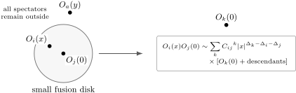
The radial OPE about zero converges when a centered sphere separates the fused pair from every spectator. This schematic planar section uses $x=(-0.52,0.28)$, $R=1.1$ and the displayed spectator $y=(0.25,1.55)$, satisfying $|x|<R<|y|$; every additional spectator must satisfy the same outside condition. The circle represents a section of the radial-quantization sphere, not a physical interaction boundary.

The relation between the three-point coefficient and the OPE coefficient is especially transparent in an orthonormal Hermitian scalar basis. Insert the OPE into a three-point function with $O_k(y)$:

$$\langle O_i(x)O_j(0)O_k(y)\rangle \sim C_{ij}{}^k |x|^{\Delta_k-\Delta_i-\Delta_j} \langle O_k(0)O_k(y)\rangle+\cdots.$$

Since

$$\langle O_k(0)O_k(y)\rangle={1\over |y|^{2\Delta_k}},$$

the leading OPE prediction is

$$\langle O_i(x)O_j(0)O_k(y)\rangle \sim {C_{ij}{}^k |x|^{\Delta_k-\Delta_i-\Delta_j} \over |y|^{2\Delta_k}}.$$

Now take the exact three-point function and let $x\to0$:

$$\langle O_i(x)O_j(0)O_k(y)\rangle ={C_{ijk}\over |x|^{\Delta_i+\Delta_j-\Delta_k} |y|^{\Delta_j+\Delta_k-\Delta_i} |y-x|^{\Delta_i+\Delta_k-\Delta_j}}$$ $$\sim {C_{ijk}|x|^{\Delta_k-\Delta_i-\Delta_j} \over |y|^{2\Delta_k}}.$$

Therefore, with orthonormal two-point functions,

$$\boxed{C_{ij}{}^k=C_{ijk}.}$$

With a general two-point metric $g_{ij}$, the raised-index coefficient is

$$C_{ij}{}^k=C_{ij\ell}g^{\ell k}, \qquad g^{\ell k}g_{km}=\delta^\ell{}_m.$$

The identity operator deserves special mention. For a Hermitian operator in a basis normalized as $\langle O_i(x)O_j(0)\rangle=\delta_{ij}/|x|^{2\Delta_i}$,

$$O_i(x)O_i(0)\sim {1\over |x|^{2\Delta_i}}\mathbf 1+\cdots.$$

The identity contribution is the most singular term in many OPEs. For a charged operator, the analogous identity term occurs in $O_i(x)O_i^\dagger(0)$ rather than necessarily in $O_i(x)O_i(0)$.

The first descendant coefficient

It is useful to see once how descendants are fixed. Consider the scalar contribution of $O_k$ in the OPE

$$O_i(x)O_j(0) \sim C_{ijk}|x|^{\Delta_k-\Delta_i-\Delta_j} \left[O_k(0)+a\,x^\mu\partial_\mu O_k(0)+\cdots\right].$$

Insert $O_k(y)$ and use

$$\partial_{0\mu}{1\over |y-0|^{2\Delta_k}} =2\Delta_k {y_\mu\over |y|^{2\Delta_k+2}}.$$

The OPE then predicts

$$\langle O_i(x)O_j(0)O_k(y)\rangle \sim {C_{ijk}|x|^{\Delta_k-\Delta_i-\Delta_j}\over |y|^{2\Delta_k}} \left[1+2a\Delta_k{x\cdot y\over y^2}+\cdots\right].$$

The exact three-point function gives, for small $x$,

$$|y-x|^{-(\Delta_i+\Delta_k-\Delta_j)} =|y|^{-(\Delta_i+\Delta_k-\Delta_j)} \left[1+(\Delta_i+\Delta_k-\Delta_j){x\cdot y\over y^2}+\cdots\right].$$

Matching the two expansions yields

$$\boxed{ a={\Delta_i-\Delta_j+\Delta_k\over 2\Delta_k} }$$

for $\Delta_k\ne0$. The global identity family is a special case because the identity has no nonzero derivative descendant. The two-dimensional Virasoro identity family is larger: it includes the stress tensor, which is not a derivative of the identity.

This calculation captures the general logic of conformal descendants: the three-point coefficient chooses the primary family, and conformal symmetry fills in the derivative tower.

Four-point factorization and conformal blocks

Apply the OPE to a four-point function in the $12$ channel:

$$O_1(x_1)O_2(x_2) \sim \sum_p C_{12}{}^p(x_{12},\partial_{x_2})O_p(x_2).$$

A second OPE can be applied to the $34$ pair. The result has the schematic form

$$\langle O_1O_2O_3O_4\rangle = \sum_p C_{12p}C_{34p}\,\mathcal G_p^{(12)(34)}(u,v),$$

up to the chosen external prefactor and with conjugate representations and spin indices paired as required. Here $\mathcal G_p$ is a global conformal block. It is fixed by the spacetime dimension, external dimensions and exchanged dimension/spin; the OPE coefficients carry the dynamics. In the reflection-even two-dimensional $u,v$ shorthand, pair the opposite-spin global contributions; a single chiral block still retains its orientation variables. Regrouping global families into Virasoro blocks additionally uses the central charge and holomorphic/antiholomorphic weights. A consistent decomposition must specify which family basis it uses; see Pappadopulo et al. 2012, revised preprint v3 (2015), p. 3, footnote 2, PDF.

This statement should feel familiar from several earlier parts of the course. In statistical mechanics, it says that short-distance clusters can be replaced by effective local insertions. In QFT language, it resembles inserting a complete set of states. In two-dimensional radial quantization, these viewpoints become literally the same: the OPE is the short-distance version of Hilbert-space completeness on a circle surrounding the fused operators.

Associativity and crossing symmetry

The OPE is a local multiplication law. A multiplication law must be associative if it is to give unambiguous correlation functions. For three nearby operators, associativity says that fusing $O_i$ with $O_j$ first and then with $O_k$ must agree with fusing $O_j$ with $O_k$ first and then with $O_i$, wherever both expansions converge after analytic continuation.

For four-point functions this becomes crossing symmetry. Each channel expansion converges in its own radial domain, and analytic continuation must reconstruct one and the same correlator. In the equation below every channel block is expressed with one common external prefactor, so any channel-dependent crossing powers are included in the definition of $\mathcal G^{(ab)(cd)}$. The $(12)(34)$, $(13)(24)$, and $(14)(23)$ decompositions then obey

$$\begin{aligned} \sum_p C_{12p}C_{34p}\,\mathcal G_p^{(12)(34)}(u,v) &= \sum_q C_{13q}C_{24q}\,\mathcal G_q^{(13)(24)}(u,v) \\ &= \sum_r C_{14r}C_{23r}\,\mathcal G_r^{(14)(23)}(u,v). \end{aligned}$$

Compare the three pairings in the figure. Each panel represents a complete sum over its intermediate families, with the same external prefactor used in all panels.

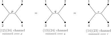
Crossing equates the full $(12)(34)$, $(13)(24)$ and $(14)(23)$ channel sums, not individual exchanged blocks. The trees show pairings and intermediate families schematically; their positions are not spacetime coordinates and their lines are not Feynman propagators. Blocks include the channel conversion to one common external prefactor; their $(u,v)$ arguments are suppressed only in the drawing.

For identical scalar primaries with

$$\langle O_1O_2O_3O_4\rangle ={1\over x_{12}^{2\Delta}x_{34}^{2\Delta}}F(u,v),$$

exchanging $x_1\leftrightarrow x_3$ gives

$$\boxed{ F(u,v)=\left({u\over v}\right)^\Delta F(v,u). }$$

For an orientation-sensitive two-dimensional correlator, the same permutation instead reads

$$\mathscr F(\eta,\bar\eta) =\left|\frac{\eta}{1-\eta}\right|^{2\Delta} \mathscr F(1-\eta,1-\bar\eta).$$

The permutation transforms the orientation branch along with the cross ratios; it does not impose reflection invariance.

This is a simple example of a bootstrap equation. It is simple to write and hard to satisfy. The equality compares two different infinite sums over exchanged primary families. In a consistent CFT, the spectrum and OPE coefficients must make all such equalities true.

The relation to Lie algebras is a useful preview. Suppose singular OPEs define modes $A_n$ by contour integrals. Then different ways of nesting OPEs become different ways of nesting commutators. Associativity of the OPE becomes the Jacobi identity,

$$[A_i,[A_j,A_k]]+[A_j,[A_k,A_i]]+[A_k,[A_i,A_j]]=0.$$

This is the mechanism behind the Virasoro algebra and current algebras in two-dimensional CFT. The algebra is not imposed from the outside; it is the short-distance consistency of local fields.

Example: Ising fusion rules

The diagonal, local two-dimensional critical Ising CFT has central charge $c=1/2$ and three Virasoro primary families:

$$\mathbf 1, \qquad \sigma, \qquad \varepsilon,$$

with dimensions

$$\Delta_{\mathbf 1}=0, \qquad \Delta_\sigma={1\over8}, \qquad \Delta_\varepsilon=1.$$

Their weights are $(h,\bar h)=(0,0)$, $(1/16,1/16)$ and $(1/2,1/2)$. These are not only three global conformal families: for example, the stress tensors belong to the Virasoro identity family. The fusion rules enumerate allowed Virasoro representations,

$$\sigma\times\sigma=\mathbf 1+\varepsilon,$$ $$\sigma\times\varepsilon=\sigma,$$ $$\varepsilon\times\varepsilon=\mathbf 1.$$

With the standard normalization

$$\langle \sigma(x)\sigma(0)\rangle={1\over |x|^{1/4}}, \qquad \langle \varepsilon(x)\varepsilon(0)\rangle={1\over |x|^{2}},$$

the remaining sign must be matched to the thermal perturbation. Retain Lesson 12’s convention $S=S_*+\tau\int\varepsilon$, $\varepsilon=-2\pi uv$, $m=2\pi\tau$, with $\tau>0$ in the ordered phase of the original lattice spin. Then the first OPE begins as

$$\sigma(x)\sigma(0) \sim {1\over |x|^{1/4}} \left[\mathbf 1-{1\over2}|x|\,\varepsilon(0)+\cdots\right].$$

The power of the identity term is fixed by

$$\Delta_{\mathbf 1}-2\Delta_\sigma=-{1\over4}.$$

The power of the energy term is fixed by

$$\Delta_\varepsilon-2\Delta_\sigma=1-{1\over4}={3\over4},$$

which is the same as the factored form $|x|^{-1/4}\cdot |x|$. Crossing fixes the coefficient’s magnitude, not its sign. One can see the magnitude from the exact Ising four-spin blocks. Define the insertion at infinity by $\sigma(\infty)=\lim_{|w|\to\infty}|w|^{1/4}\sigma(w)$ inside correlators. For $G_4(z,\bar z)=\langle\sigma(0)\sigma(z,\bar z)\sigma(1)\sigma(\infty)\rangle$, choose branches continuously from $0<z<1$:

$$\mathcal F_\pm(z) =[z(1-z)]^{-1/8} \sqrt{\frac{1\pm\sqrt{1-z}}{2}}, \qquad G_4(z,\bar z)=|\mathcal F_+(z)|^2+|\mathcal F_-(z)|^2.$$

These are the plane blocks for $c=1/2$, $h_\sigma=1/16$. They solve the null-vector equation; deriving that equation is beyond this first OPE lesson. The radical solutions and their coordinate prefactor are given in Di Francesco, Mathieu and Sénéchal 1997, Exercise 8.12(d–e), pp. 287–288, and § 11.2, p. 418. Here the energy-channel block includes its coefficient, so it is not normalized to unit leading term. Expanding directly gives

$$\mathcal F_+(z)=z^{-1/8}\bigl[1+O(z^2)\bigr], \qquad \mathcal F_-(z)=\frac12 z^{3/8}\bigl[1+O(z)\bigr].$$

The energy channel therefore contributes $\tfrac14|z|^{3/4}$ to $G_4$, while the identity contributes $|z|^{-1/4}$. Thus $C_{\sigma\sigma\varepsilon}^2=1/4$. The textbook independently obtains this square and chooses the positive sign only after allowing an energy-field redefinition in Di Francesco, Mathieu and Sénéchal 1997, § 12.3.3, p. 451, Eqs. (12.63)–(12.64).

The sign in this course follows from its lattice-to-thermal identification. On a finite zero-field ferromagnetic graph, a bond coupling obeys

$$\partial_{K_{ij}}\langle s_xs_y\rangle =\langle s_xs_y\,s_is_j\rangle_c\ge0.$$

The nonnegative covariance has a direct two-replica proof. For independent spin configurations $s,t$, set $a_i=(s_i+t_i)/2$ and $b_i=(s_i-t_i)/2$. The product Gibbs weight has bond factors $\exp[2K_{ij}(a_ia_j+b_ib_j)]$, with $K_{ij}\ge0$. The covariance is one-half the expectation of $(s_xs_y-t_xt_y)(s_is_j-t_it_j)$. Each difference is a sum with positive coefficients, for example $s_xs_y-t_xt_y=2(a_xb_y+b_xa_y)$. Expand the bond exponentials: every coefficient is nonnegative, and the independent single-site sum over $(a_i,b_i)=(\pm1,0),(0,\pm1)$ kills odd or mixed powers while leaving nonnegative even powers. The convergent finite-graph expansion therefore proves the inequality.

The lattice action changes by $-\delta K\sum_b s_is_j$, whereas positive $\tau\int\varepsilon$ moves in that same ordered direction. Hence the leading scalar part of the centered bond has a negative coefficient of $\varepsilon$. At separated points in the critical scaling limit, its nonnegative covariance with two order spins requires $C_{\sigma\sigma\varepsilon}\le0$; the nonzero crossing magnitude fixes $C_{\sigma\sigma\varepsilon}=-1/2$. Centering removes identity mixing, and separated insertions avoid contact terms. Simultaneously replacing $\varepsilon\to-\varepsilon$ and $\tau\to-\tau$ gives the familiar positive coefficient and reverses the sign of the thermal coupling; changing the sign of $\sigma$ alone cannot change it.

The disorder operator $\mu$ belongs to the same Virasoro representation as $\sigma$ and has the same dimension,

$$\Delta_\mu={1\over8},$$

and it obeys the same family-level rule $\mu\times\mu=\mathbf 1+\varepsilon$. Duality reverses the thermal field, so $C_{\mu\mu\varepsilon}=-C_{\sigma\sigma\varepsilon}=+1/2$ in the convention above. The opposite coefficients and the order/disorder construction are discussed in Di Francesco, Mathieu and Sénéchal 1997, § 12.2, pp. 443–445. The disorder field is not an additional mutually local primary of the diagonal three-primary theory: it is defined at the endpoint of a disorder line. Its mutual locality with $\sigma$ therefore differs, and the mixed OPE $\sigma\times\mu$ contains fermionic fields with branch-cut behavior. Family fusion rules list allowed representations; their plus signs do not specify numerical OPE signs.

Two-dimensional notation

In two Euclidean dimensions, write

$$z=x^1+i x^2, \qquad \bar z=x^1-i x^2.$$

A local conformal map is

$$z'=f(z), \qquad \bar z'=\bar f(\bar z),$$

and the metric transforms as

$$dz' d\bar z'=f'(z)\bar f'(\bar z)\,dz d\bar z.$$

A primary field with holomorphic and antiholomorphic weights $(h,\bar h)$ transforms as

$$O'(z',\bar z') =\left(f'(z)\right)^{-h} \left(\bar f'(\bar z)\right)^{-\bar h} O(z,\bar z).$$

Its scaling dimension and spin are

$$\Delta=h+\bar h, \qquad s=h-\bar h.$$

For spinless fields $h=\bar h=\Delta/2$. The two-point function becomes

$$\langle O_i(z_1,\bar z_1)O_j(z_2,\bar z_2)\rangle ={\delta_{ij}\over z_{12}^{2h_i}\bar z_{12}^{2\bar h_i}}$$

in an orthonormal basis. The three-point function factorizes similarly into a holomorphic power law times an antiholomorphic power law. The next pages exploit this holomorphic structure and eventually turn the stress tensor into an infinite set of generators.

Summary

Conformal symmetry fixes scalar two- and three-point functions up to constants. In an orthonormal conformal basis,

$$\langle O_i(x)O_j(0)\rangle={\delta_{ij}\over |x|^{2\Delta_i}},$$

and

$$\langle O_1(x_1)O_2(x_2)O_3(x_3)\rangle ={C_{123}\over x_{12}^{\Delta_1+\Delta_2-\Delta_3} x_{23}^{\Delta_2+\Delta_3-\Delta_1} x_{13}^{\Delta_1+\Delta_3-\Delta_2}}.$$

Four-point functions contain arbitrary functions of cross ratios, but these functions are not arbitrary in a consistent theory. The OPE decomposes a four-point function into conformal blocks with coefficients determined by three-point data. Associativity of the OPE requires equality of different channel decompositions. This is crossing symmetry, the central consistency condition of conformal bootstrap.

Common pitfalls

Confusing dimensions with OPE coefficients. Symmetry fixes the powers of $x_{ij}$, but it does not in general fix the constants $C_{ijk}$. Dimensions and OPE coefficients are independent pieces of CFT data constrained jointly by crossing.

Using the wrong convergence center. The displayed OPE expands about zero and requires $|x|<\min_a|y_a|$. An off-center sphere that happens to enclose the pair does not prove this condition. Radial quantization gives convergence in the stated CFT domain; generic QFTs can require an asymptotic formulation.

Dropping the identity family. The identity contribution often dominates the short-distance limit. Forgetting it gives the wrong leading singularity and usually spoils the disconnected part of a four-point function.

Treating the reduced correlator as convention independent. A four-point function can be written with many different kinematic prefactors. The function called $F(u,v)$ changes with that choice, while the full correlator and its crossing content do not.

Reducing crossing to a relabeling. Crossing equates different OPE sums, generally organized around different limits and convergence regions. The equality therefore imposes dynamical constraints on the spectrum and OPE coefficients.

Exercises

Exercise 1: Three-point exponents from inversion

Derive the conformal form of a scalar three-point function by starting from

$$G_3={C_{123}\over x_{12}^{a}x_{23}^{b}x_{13}^{c}}$$

and imposing inversion covariance. For this exercise additionally assume the vacuum is invariant under inversion and the scalar primaries are inversion-even without operator mixing.

Solution

Under inversion,

$$x_{ij}'={x_{ij}\over (x_i^2x_j^2)^{1/2}}.$$

Thus

$$G_3(x_i') ={C_{123} (x_1^2)^{(a+c)/2} (x_2^2)^{(a+b)/2} (x_3^2)^{(b+c)/2} \over x_{12}^{a}x_{23}^{b}x_{13}^{c}}.$$

Primary covariance requires

$$G_3(x_i') =(x_1^2)^{\Delta_1}(x_2^2)^{\Delta_2}(x_3^2)^{\Delta_3}G_3(x_i).$$

Therefore

$${a+c\over2}=\Delta_1, \qquad {a+b\over2}=\Delta_2, \qquad {b+c\over2}=\Delta_3.$$

Solving gives

$$a=\Delta_1+\Delta_2-\Delta_3,$$ $$b=\Delta_2+\Delta_3-\Delta_1,$$ $$c=\Delta_1+\Delta_3-\Delta_2.$$

Substitution gives the three-point formula in the main text.

Exercise 2: Invariance of the cross ratios

Show that

$$u={x_{12}^2x_{34}^2\over x_{13}^2x_{24}^2}, \qquad v={x_{14}^2x_{23}^2\over x_{13}^2x_{24}^2}$$

are invariant under inversion.

Solution

Inversion sends

$$x_{ij}^2\mapsto x_{ij}'{}^2={x_{ij}^2\over x_i^2x_j^2}.$$

For $u$ this gives

$$u' ={x_{12}^2(x_1^2x_2^2)^{-1}x_{34}^2(x_3^2x_4^2)^{-1} \over x_{13}^2(x_1^2x_3^2)^{-1}x_{24}^2(x_2^2x_4^2)^{-1}}.$$

The factors $x_1^2x_2^2x_3^2x_4^2$ cancel, leaving

$$u'=u.$$

The calculation for $v$ is identical:

$$v' ={x_{14}^2(x_1^2x_4^2)^{-1}x_{23}^2(x_2^2x_3^2)^{-1} \over x_{13}^2(x_1^2x_3^2)^{-1}x_{24}^2(x_2^2x_4^2)^{-1}} =v.$$

Exercise 3: Three-point data from the OPE

Assume an orthonormal Hermitian scalar basis. Use the OPE to show that the leading coefficient in

$$O_i(x)O_j(0)\sim\sum_k C_{ij}{}^k |x|^{\Delta_k-\Delta_i-\Delta_j}O_k(0)+\cdots$$

is equal to the three-point coefficient $C_{ijk}$.

Solution

Insert both sides into a correlator with $O_k(y)$. The OPE gives

$$\langle O_i(x)O_j(0)O_k(y)\rangle \sim C_{ij}{}^k |x|^{\Delta_k-\Delta_i-\Delta_j} \langle O_k(0)O_k(y)\rangle.$$

Using the orthonormal two-point function,

$$\langle O_k(0)O_k(y)\rangle={1\over |y|^{2\Delta_k}},$$

we get

$$\langle O_i(x)O_j(0)O_k(y)\rangle \sim {C_{ij}{}^k |x|^{\Delta_k-\Delta_i-\Delta_j}\over |y|^{2\Delta_k}}.$$

The exact three-point function is

$${C_{ijk}\over |x|^{\Delta_i+\Delta_j-\Delta_k} |y|^{\Delta_j+\Delta_k-\Delta_i} |y-x|^{\Delta_i+\Delta_k-\Delta_j}}.$$

Taking $x\to0$ gives

$${C_{ijk}|x|^{\Delta_k-\Delta_i-\Delta_j}\over |y|^{2\Delta_k}}.$$

Matching the two expressions gives

$$C_{ij}{}^k=C_{ijk}.$$

Exercise 4: The first scalar descendant

Find the coefficient $a$ of the first derivative descendant in

$$O_i(x)O_j(0) \sim C_{ijk}|x|^{\Delta_k-\Delta_i-\Delta_j} \left[O_k(0)+a x^\mu\partial_\mu O_k(0)+\cdots\right].$$

Assume $\Delta_k\ne0$.

Solution

Insert $O_k(y)$. The derivative acts on the two-point function as

$$\partial_{0\mu}|y|^{-2\Delta_k} =2\Delta_k {y_\mu\over |y|^{2\Delta_k+2}}.$$

The OPE therefore predicts

$${C_{ijk}|x|^{\Delta_k-\Delta_i-\Delta_j}\over |y|^{2\Delta_k}} \left[1+2a\Delta_k{x\cdot y\over y^2}+\cdots\right].$$

The exact three-point function contains the factor

$$|y-x|^{-(\Delta_i+\Delta_k-\Delta_j)}.$$

For small $x$,

$$|y-x|^{-A}=|y|^{-A} \left[1+A{x\cdot y\over y^2}+\cdots\right], \qquad A=\Delta_i+\Delta_k-\Delta_j.$$

Matching the coefficient of $x\cdot y/y^2$ gives

$$2a\Delta_k=\Delta_i+\Delta_k-\Delta_j.$$

Thus

$$\boxed{ a={\Delta_i-\Delta_j+\Delta_k\over 2\Delta_k}. }$$

Exercise 5: Identical-scalar crossing equation

For identical scalar primaries in $d\ge3$, or for a reflection-even two-dimensional correlator, derive the crossing relation

$$F(u,v)=\left({u\over v}\right)^\Delta F(v,u)$$

from the equality of the four-point function under $x_1\leftrightarrow x_3$.

Solution

Write

$$G_4(x_1,x_2,x_3,x_4) ={1\over x_{12}^{2\Delta}x_{34}^{2\Delta}}F(u,v).$$

Exchanging $x_1$ and $x_3$ sends $u\leftrightarrow v$ and gives

$$G_4(x_3,x_2,x_1,x_4) ={1\over x_{23}^{2\Delta}x_{14}^{2\Delta}}F(v,u).$$

For identical operators the two correlators are equal. Hence

$${F(u,v)\over x_{12}^{2\Delta}x_{34}^{2\Delta}} = {F(v,u)\over x_{23}^{2\Delta}x_{14}^{2\Delta}}.$$

Multiplying through gives

$$F(u,v)= \left({x_{12}^2x_{34}^2\over x_{23}^2x_{14}^2}\right)^\Delta F(v,u).$$

Using

$${u\over v}={x_{12}^2x_{34}^2\over x_{14}^2x_{23}^2},$$

we obtain

$$F(u,v)=\left({u\over v}\right)^\Delta F(v,u).$$

Exercise 6: Ising short-distance powers

Use the Ising dimensions $\Delta_\sigma=1/8$ and $\Delta_\varepsilon=1$ to determine the powers of $|x|$ in the identity and energy contributions to $\sigma(x)\sigma(0)$.

Solution

The scalar OPE power for an exchanged operator $O_k$ is

$$|x|^{\Delta_k-\Delta_i-\Delta_j}.$$

For $\sigma(x)\sigma(0)$, $\Delta_i=\Delta_j=\Delta_\sigma=1/8$.

For the identity, $\Delta_{\mathbf 1}=0$, so

$$\Delta_{\mathbf 1}-2\Delta_\sigma=0-{1\over4}=-{1\over4}.$$

Thus the identity contribution scales as

$$|x|^{-1/4}\mathbf 1.$$

For the energy operator,

$$\Delta_\varepsilon-2\Delta_\sigma=1-{1\over4}={3\over4}.$$

Thus the energy contribution scales as

$$|x|^{3/4}\varepsilon(0).$$

Factoring out the leading identity singularity gives

$$\sigma(x)\sigma(0) \sim |x|^{-1/4}\left[\mathbf 1+C_{\sigma\sigma\varepsilon}|x|\varepsilon(0)+\cdots\right].$$

Unit two-point normalization and crossing give $|C_{\sigma\sigma\varepsilon}|=1/2$. With Lesson 12’s positive thermal coupling pointing into the ordered phase, $C_{\sigma\sigma\varepsilon}=-1/2$; the powers are unchanged by this convention choice.

References

• Di Francesco, Philippe, Pierre Mathieu, and David Sénéchal. Conformal Field Theory. Graduate Texts in Contemporary Physics. New York: Springer, 1997. DOI.
• Pappadopulo, Duccio, Slava Rychkov, Johnny Espin, and Riccardo Rattazzi. “OPE Convergence in Conformal Field Theory.” Physical Review D 86 (2012): 105043. DOI. Open PDF: arXiv v3, revised 12 June 2015.

Further reading

• Kelly, Douglas G., and Seymour Sherman. “General Griffiths’ Inequalities on Correlations in Ising Ferromagnets.” Journal of Mathematical Physics 9 (1968): 466–484. DOI. The general correlation inequalities extend the finite zero-field argument given above.
• Rychkov, Slava. EPFL Lectures on Conformal Field Theory in D ≥ 3 Dimensions. SpringerBriefs in Physics. Cham: Springer, 2017. DOI. Open PDF: 2016 arXiv v2.