Feynman Propagator and the iε Prescription

The previous page showed that the time-ordered two-point function is a Green function. For a harmonic oscillator,

$$\left(\frac{d^2}{dt^2}+\omega_0^2\right) \langle0|\mathcal T q(t)q(t')|0\rangle=-i\delta(t-t'),$$

and for a real scalar field,

$$(\Box_x+m^2)\langle0|\mathcal T\phi(x)\phi(y)|0\rangle =-i\delta^{(4)}(x-y).$$

But a differential equation plus a delta-function source still does not uniquely determine the propagator. We may add any homogeneous solution. In momentum space this ambiguity is exactly the ambiguity of what to do with the poles. The Feynman propagator is the inverse selected by the time-ordered vacuum expectation value: positive-energy modes propagate forward in time, negative-energy modes propagate backward in time, and the pole prescription encodes both statements in one compact formula.

The result is so small that it is easy to underestimate:

$$\boxed{ G_F(x-y)=\langle0|\mathcal T\phi(x)\phi(y)|0\rangle =\int\frac{d^4p}{(2\pi)^4}\, \frac{i\,e^{-ip\cdot(x-y)}}{p^2-m^2+i\epsilon} }$$

with $\epsilon>0$ and the limit $\epsilon\to0^+$ taken after integration. This page explains what that $i\epsilon$ means.

Three equivalent ways to recognize the same object

This course lesson preserves an oscillator-first derivation and its lecture sequence. Scalar Propagators, Ordered Correlators, and Sources develops the field-theory inverse and source normalization, while Lorentzian Boundary Conditions and iε compares vacuum selection, causal prescriptions, and Wick-rotation qualifications.

Feynman boundary value and factor of i

We keep the global mostly-minus convention $p^2=(p^0)^2-\mathbf p^2$. The qft.org convention page denotes the scalar Feynman propagator by $D_F$; here we write $G_F$ for the same object when emphasizing its role as a Green function, so $G_F=D_F$ in these conventions. For the oscillator warm-up, the frequency is denoted by $\omega_0>0$, while $\omega$ is the Fourier variable. The oscillator Feynman two-point function is

$$G_F(t-t')=\langle0|\mathcal Tq(t)q(t')|0\rangle,$$

with no extra factor of $i$ removed. With this choice,

$$G_F(\tau)=\int\frac{d\omega}{2\pi}\, \frac{i\,e^{-i\omega\tau}}{\omega^2-\omega_0^2+i\epsilon}.$$

Other common conventions define a Green function with an extra factor of $i$ removed, write the mostly-plus metric, or assign the symbol $D_F$ differently. Those conventions move names, signs, and factors of $i$, but the pole displacement is the same physical prescription. The safest local test in the present convention is always

$$(\partial_\tau^2+\omega_0^2)G_F(\tau)=-i\delta(\tau), \qquad (\Box+m^2)G_F(x)=-i\delta^{(4)}(x).$$

Those two equations fix the normalization used below.

Before doing contour integrals, keep three descriptions of the Feynman propagator in view. They are mathematically equivalent, but each one prevents a different mistake.

Description	Formula	What it fixes
Operator definition	$G_F(x-y)=\langle0	\mathcal T\phi(x)\phi(y)
Green-function equation	$(\Box_x+m^2)G_F(x-y)=-i\delta^{(4)}(x-y)$	the local differential operator being inverted
Momentum-space distribution	$G_F(p)=i/(p^2-m^2+i0)$	how the poles are bypassed

The second line alone is not enough. A Green function is an inverse plus a boundary condition. The $i0$ prescription is that boundary condition written in momentum space. Whenever a later calculation contains a denominator such as $p^2-m^2$, the invisible question is always: which side of the pole are we on?

Spectral construction of the time-ordered oscillator propagator

Start with one harmonic oscillator,

$$q(t)=e^{iHt}q(0)e^{-iHt}, \qquad H|n\rangle=E_n|n\rangle, \qquad E_n\ge E_0.$$

For $t>t'$, time ordering does nothing:

$$G_F(t,t')=\langle0|q(t)q(t')|0\rangle.$$

Insert a complete set of energy eigenstates between the two operators:

$$\begin{aligned} G_F(t,t') &=\sum_n \langle0|q(t)|n\rangle\langle n|q(t')|0\rangle \\ &=\sum_n \langle0|e^{iHt}q(0)e^{-iHt}|n\rangle \langle n|e^{iHt'}q(0)e^{-iHt'}|0\rangle \\ &=\sum_n |\langle0|q(0)|n\rangle|^2 e^{-i(E_n-E_0)(t-t')}. \end{aligned}$$

For $t<t'$, the ordered product is reversed:

$$G_F(t,t')=\langle0|q(t')q(t)|0\rangle =\sum_n |\langle0|q(0)|n\rangle|^2 e^{+i(E_n-E_0)(t-t')}.$$

Thus, in terms of $\tau=t-t'$,

$$G_F(\tau)=\theta(\tau) \sum_n |\langle0|q|n\rangle|^2e^{-i(E_n-E_0)\tau} +\theta(-\tau) \sum_n |\langle0|q|n\rangle|^2e^{+i(E_n-E_0)\tau}.$$

This expression is already the Feynman boundary condition. When $\tau>0$, only positive-energy excitations move from the earlier insertion to the later insertion. When $\tau<0$, the time-ordered product reverses the operators, giving the corresponding negative-frequency piece in the variable $\tau$.

For a single oscillator, only the one-particle state contributes because

$$q=\frac{1}{\sqrt{2\omega_0}}(a+a^\dagger), \qquad a|0\rangle=0,$$

so

$$|\langle0|q|1\rangle|^2=\frac{1}{2\omega_0}.$$

Therefore

$$\boxed{ G_F(\tau)=\frac{1}{2\omega_0}e^{-i\omega_0|\tau|} }$$

which is the same Green function derived from contact terms on the previous page.

Fourier transform and the pole ambiguity

Write the Fourier transform as

$$G_F(\tau)=\int_{-\infty}^{\infty}\frac{d\omega}{2\pi}\, e^{-i\omega\tau}\widetilde G_F(\omega), \qquad \widetilde G_F(\omega)=\int_{-\infty}^{\infty}d\tau\, e^{i\omega\tau}G_F(\tau).$$

Using the spectral form, the $\tau>0$ part gives

$$\int_0^\infty d\tau\, e^{i\omega\tau}e^{-i(E_n-E_0)\tau}$$

which is not an ordinary convergent integral. The time-ordered vacuum expectation value tells us how to regularize it: insert a damping factor $e^{-\epsilon\tau}$ with $\epsilon>0$ and take $\epsilon\to0^+$ at the end. Then

$$\int_0^\infty d\tau\, e^{i(\omega-E)\tau}e^{-\epsilon\tau} =\frac{i}{\omega-E+i\epsilon}.$$

The $\tau<0$ part is damped by $e^{+\epsilon\tau}$, so

$$\int_{-\infty}^{0}d\tau\, e^{i(\omega+E)\tau}e^{+\epsilon\tau} =-\frac{i}{\omega+E-i\epsilon}.$$

Thus the spectral representation of the oscillator Feynman propagator is

$$\widetilde G_F(\omega) =\sum_n |\langle0|q|n\rangle|^2 \left[ \frac{i}{\omega-(E_n-E_0)+i\epsilon} -\frac{i}{\omega+(E_n-E_0)-i\epsilon} \right].$$

For the harmonic oscillator, $E_1-E_0=\omega_0$ and the matrix element is $1/(2\omega_0)$. Hence

$$\begin{aligned} \widetilde G_F(\omega) &=\lim_{\epsilon\to0^+}\frac{1}{2\omega_0} \left[ \frac{i}{\omega-\omega_0+i\epsilon} -\frac{i}{\omega+\omega_0-i\epsilon} \right] \\ &=\frac{i}{\omega^2-\omega_0^2+i0}. \end{aligned}$$

The limit sign matters. At finite $\epsilon$, the first line combines algebraically to

$$\frac{i+\epsilon/\omega_0} {\omega^2-\omega_0^2+2i\omega_0\epsilon+\epsilon^2},$$

not to the same expression with a literal $+i\epsilon$ in the quadratic denominator. The linear regulator has units of frequency, whereas a regulator added to $\omega^2-\omega_0^2$ has units of frequency squared. Both give the same boundary-value distribution as $\epsilon\to0^+$ after a positive rescaling. Accordingly, the compact notation

$$\omega^2-\omega_0^2+i0$$

is the distributional shorthand

$$\left(\omega-\omega_0+i0\right) \left(\omega+\omega_0-i0\right),$$

where the precise positive scale multiplying each $0$ is irrelevant. What matters is the side of the real axis, not an equality between finite regulators. The positive-frequency pole is below the real axis and the negative-frequency pole is above it:

$$\omega=+\omega_0-i0, \qquad \omega=-\omega_0+i0.$$

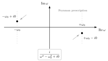
The Feynman prescription displaces the positive-frequency pole below the real $\omega$ axis and the negative-frequency pole above it. This is the contour-language version of the time-ordered vacuum boundary condition.

The sign is worth memorizing:

$$\boxed{ \frac{i}{\omega^2-\omega_0^2+i\epsilon} \quad\Longleftrightarrow\quad \omega=+\omega_0-i0,\; -\omega_0+i0. }$$

The two poles are not shifted in the same direction. That split is what makes the propagator Feynman rather than retarded or advanced.

A practical warning: the symbol $+i\epsilon$ should not be cancelled too early. It is not an ordinary small correction to the mass. It is a rule for how to pass the poles before the Fourier integral is done. After the contour has been chosen, the limit $\epsilon\to0^+$ may be taken.

Evaluating the contour integral

A reliable contour calculation has only three decisions:

1. factor the denominator and mark the displaced poles;
2. choose the half-plane where $e^{-i\omega\tau}$ decays;
3. remember the orientation of the closed contour.

The sign errors in this subject usually come from skipping step 3. Closing below is clockwise, so it contributes $-2\pi i$ times the enclosed residues; closing above is counterclockwise, so it contributes $+2\pi i$ times the enclosed residues.

Now verify directly that

$$G_F(\tau)=\int\frac{d\omega}{2\pi}\, \frac{i e^{-i\omega\tau}}{\omega^2-\omega_0^2+i\epsilon}$$

reproduces $G_F(\tau)=e^{-i\omega_0|\tau|}/(2\omega_0)$.

For $\tau>0$, the factor $e^{-i\omega\tau}$ decays in the lower half-plane. Indeed, if $\omega=u+iv$, then

$$e^{-i\omega\tau}=e^{-iu\tau}e^{v\tau},$$

so for $\tau>0$ we need $v<0$. Closing the contour below encloses only the pole at $\omega=+\omega_0-i0$. The contour is clockwise, giving

$$G_F(\tau>0) =-i\operatorname*{Res}_{\omega=\omega_0} \frac{i e^{-i\omega\tau}}{(\omega-\omega_0)(\omega+\omega_0)} =\frac{1}{2\omega_0}e^{-i\omega_0\tau}.$$

For $\tau<0$, the exponential decays in the upper half-plane. Closing above encloses only the pole at $\omega=-\omega_0+i0$, and the contour is counterclockwise:

$$G_F(\tau<0) =+i\operatorname*{Res}_{\omega=-\omega_0} \frac{i e^{-i\omega\tau}}{(\omega-\omega_0)(\omega+\omega_0)} =\frac{1}{2\omega_0}e^{+i\omega_0\tau}.$$

Since $\tau<0$, this is again $e^{-i\omega_0|\tau|}/(2\omega_0)$.

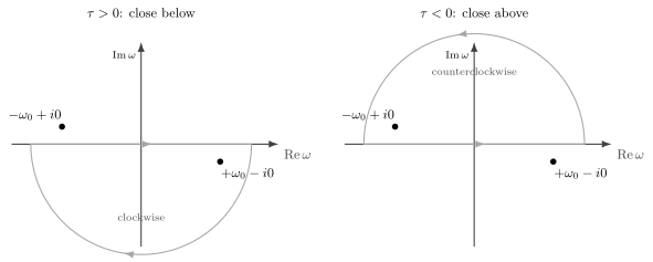
For $\tau>0$, the exponential $e^{-i\omega\tau}$ damps the lower half-plane contour, so the positive-frequency pole contributes. For $\tau<0$, the contour closes above and the negative-frequency pole contributes.

The contour computation is a useful sanity check because it ties together three statements that are often learned separately:

$$\text{time ordering} \quad\Longleftrightarrow\quad \text{vacuum spectral sums} \quad\Longleftrightarrow\quad \text{Feynman pole prescription}.$$

Complex time and vacuum boundary conditions

The small imaginary parts also have a time-domain interpretation. The spectral sum for $t>t'$ contains terms

$$e^{-i(E_n-E_0)(t-t')}.$$

For a general interacting theory there are infinitely many states, so this expression is safest if the later time is displaced slightly below the earlier time in the complex plane:

$$\operatorname{Im}(t-t')<0.$$

Then high-energy intermediate states are exponentially damped:

$$e^{-iE(a-ib)}=e^{-iEa}e^{-Eb}, \qquad b>0.$$

For $t<t'$, the time-ordered product reverses the operators, and the analogous convergence condition is reversed. The usual $i\epsilon$ prescription is a compact way of implementing this ordered complex-time separation for every pair of insertions.

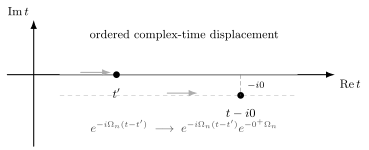
The Feynman prescription may be viewed as a tiny deformation of the time contour. Later insertions are displaced slightly lower in imaginary time, which damps high-energy intermediate states in the spectral representation.

This is also why the same symbol $i\epsilon$ appears when one projects onto the vacuum in path integrals. If the time-evolution operator is slightly tilted into the lower half-plane,

$$e^{-iH T}\longrightarrow e^{-iH T}e^{-\epsilon H T},$$

then excited states are suppressed relative to the ground state for large positive $T$. The $i\epsilon$ is not merely a trick for avoiding poles; it is the analytic memory of the vacuum boundary condition.

The scalar Feynman propagator

A free real scalar field decomposes into independent oscillator modes. Using the covariant normalization adopted in the course conventions,

$$\phi(x)=\int\frac{d^3\mathbf p}{(2\pi)^3 2E_{\mathbf p}} \left[ a(\mathbf p)e^{-ip\cdot x} +a^{\dagger}(\mathbf p)e^{ip\cdot x} \right], \qquad E_{\mathbf p}=\sqrt{\mathbf p^2+m^2},$$

with $p^0=E_{\mathbf p}$ and

$$[a(\mathbf p),a^{\dagger}(\mathbf q)] =(2\pi)^3 2E_{\mathbf p}\,\delta^{(3)}(\mathbf p-\mathbf q).$$

The same formulas can be rewritten with noncovariantly normalized oscillators and explicit factors of $1/\sqrt{2E_{\mathbf p}}$; the final two-point function is unchanged. The time-ordered two-point function is

$$G_F(x-y)=\langle0|\mathcal T\phi(x)\phi(y)|0\rangle.$$

For $x^0>y^0$,

$$G_F(x-y)=\int\frac{d^3\mathbf p}{(2\pi)^3}\frac{1}{2E_{\mathbf p}} e^{-iE_{\mathbf p}(x^0-y^0)+i\mathbf p\cdot(\mathbf x-\mathbf y)}.$$

For $x^0<y^0$,

$$G_F(x-y)=\int\frac{d^3\mathbf p}{(2\pi)^3}\frac{1}{2E_{\mathbf p}} e^{+iE_{\mathbf p}(x^0-y^0)-i\mathbf p\cdot(\mathbf x-\mathbf y)}.$$

The $p^0$ contour integral packages both cases into one Lorentz-covariant expression:

$$\boxed{ G_F(x-y)=\int\frac{d^4p}{(2\pi)^4}\, \frac{i\,e^{-ip\cdot(x-y)}}{p^2-m^2+i\epsilon} }$$

because the poles in the $p^0$ plane are

$$p^0=+E_{\mathbf p}-i0, \qquad p^0=-E_{\mathbf p}+i0.$$

This formula is one of the central pieces of perturbative QFT. Every internal scalar line in a Feynman diagram carries this factor in momentum space.

The propagator is also an inverse of the Klein–Gordon operator. Acting with $\Box_x+m^2$ gives

$$\begin{aligned} (\Box_x+m^2)G_F(x-y) &=\lim_{\epsilon\to0^+}\int\frac{d^4p}{(2\pi)^4} \frac{i(-p^2+m^2)e^{-ip\cdot(x-y)}}{p^2-m^2+i\epsilon} \\ &=-i\int\frac{d^4p}{(2\pi)^4}e^{-ip\cdot(x-y)} \\ &=-i\delta^{(4)}(x-y). \end{aligned}$$

The second line follows in the distributional limit. At nonzero $\epsilon$ there is a residual term proportional to $\epsilon/(p^2-m^2+i\epsilon)$; it vanishes as a distribution when $\epsilon\to0^+$.

Thus

$$\boxed{ (\Box_x+m^2)G_F(x-y)=-i\delta^{(4)}(x-y). }$$

The inverse and the boundary condition are both essential. The equation tells us that $G_F$ is a Green function. The $i\epsilon$ tells us which Green function.

Feynman, retarded, and advanced prescriptions

The same differential operator has several useful inverses. The difference between them is not the algebraic denominator; it is the pole placement.

The Feynman propagator places one pole below and one pole above:

$$G_F(p)=\frac{i}{(p^0)^2-E_{\mathbf p}^2+i\epsilon}.$$

The retarded propagator vanishes for $x^0<y^0$. With the same QFT normalization as $G_F$, so that the wave operator produces $-i\delta$, its poles both lie below the real axis:

$$G_R^{\mathrm{QFT}}(p)=\frac{i}{(p^0+i\epsilon)^2-E_{\mathbf p}^2}.$$

The classical response Green function usually differs by a factor $i$ or $-i$, depending on convention, because it is normalized to solve an equation with $+\delta$ on the right-hand side. Keep these two uses of the word “retarded” separate: the support property is the same, but the normalization can differ.

The advanced propagator vanishes for $x^0>y^0$. Its poles both lie above the real axis:

$$G_A^{\mathrm{QFT}}(p)=\frac{i}{(p^0-i\epsilon)^2-E_{\mathbf p}^2}.$$

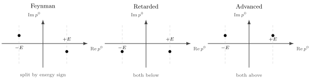
Different Green functions invert the same quadratic operator but impose different boundary conditions. Feynman poles are split by energy sign. Retarded poles are both below the real axis, so the propagator vanishes before the source. Advanced poles are both above, so the propagator vanishes after the source.

This comparison prevents a common misconception. The Feynman propagator is not the same as a classical causal response function. It is time ordered. It is the object naturally produced by vacuum correlation functions, Dyson perturbation theory, and the path integral with vacuum boundary conditions. Retarded Green functions are the natural objects for response theory and causal evolution from a source.

The difference matters already for a free field. Away from the light cone and away from coincident points, each Green function solves the homogeneous Klein–Gordon equation. Their distinctions live in boundary conditions, analytic structure, and singular support.

The distribution identity behind the prescription

A useful way to remember the prescription is the distribution identity

$$\frac{1}{x\pm i0}=\operatorname{PV}\frac{1}{x}\mp i\pi\delta(x),$$

where $\operatorname{PV}$ denotes the Cauchy principal value. Therefore

$$\frac{i}{p^2-m^2+i0} =i\operatorname{PV}\frac{1}{p^2-m^2}+\pi\delta(p^2-m^2).$$

The pole prescription is not just a way of assigning a contour; it also specifies the delta-function part supported on the mass shell. Later, when loop diagrams develop branch cuts and imaginary parts, this identity will become the local algebra behind thresholds, spectral densities, and cutting rules.

For now, the main lesson is simpler: the propagator knows about on-shell particles through its singularities. The free scalar propagator has poles at

$$p^2=m^2,$$

and the $i\epsilon$ tells us how the integration contour passes those poles.

Summary

The Feynman propagator is not merely an algebraic inverse. It is the inverse of the quadratic wave operator with the vacuum time-ordering boundary condition. In the oscillator problem,

$$G_F(\tau)=\frac{1}{2\omega_0}e^{-i\omega_0|\tau|} =\int\frac{d\omega}{2\pi}\, \frac{i e^{-i\omega\tau}}{\omega^2-\omega_0^2+i\epsilon}.$$

The $i\epsilon$ prescription means

$$+\omega_0\text{ pole below}, \qquad -\omega_0\text{ pole above}.$$

For the scalar field, the same oscillator prescription applied to every momentum mode gives

$$G_F(x-y)=\int\frac{d^4p}{(2\pi)^4}\, \frac{i e^{-ip\cdot(x-y)}}{p^2-m^2+i\epsilon}.$$

This propagator obeys

$$(\Box_x+m^2)G_F(x-y)=-i\delta^{(4)}(x-y),$$

but the Green-function equation alone does not specify it. The pole prescription supplies the vacuum boundary condition. That is why the tiny $i\epsilon$ is conceptually large: it remembers which state is the vacuum and which correlator perturbation theory computes.

Common pitfalls

The most common mistake is to write $i/(p^2-m^2)$ without specifying a prescription. That expression is not a distribution until the poles are defined.

Another frequent mistake is to think that $+i\epsilon$ moves both energy poles in the same direction. It does not. With the Feynman prescription,

$$p^0=+E_{\mathbf p}-i0, \qquad p^0=-E_{\mathbf p}+i0.$$

A third mistake is to confuse the Feynman propagator with the retarded propagator. Retarded propagation is causal in the source-response sense. Feynman propagation is time ordered and is designed for vacuum amplitudes.

Finally, $\epsilon$ is not a small physical decay rate in the free theory. It is a regulator and boundary-condition marker. Physical widths appear later when self-energy corrections move poles away from the real axis by finite imaginary parts.

A practical diagnostic: if a calculation of the free propagator gives a function symmetric under moving both poles upward or both poles downward, it is not the Feynman propagator. Feynman boundary conditions split the poles in opposite directions.

A compact denominator such as $p^2-m^2+i\epsilon$ is also a convention-dependent shorthand. Do not factor it as if the same imaginary amount were added to both roots. The correct Feynman statement is the pole placement $p^0=+E_{\mathbf p}-i0$ and $p^0=-E_{\mathbf p}+i0$.

Exercises

Exercise 1: Contour evaluation of the oscillator propagator

Evaluate

$$I(\tau)=\int_{-\infty}^{\infty}\frac{d\omega}{2\pi}\, \frac{i e^{-i\omega\tau}}{\omega^2-\omega_0^2+i\epsilon}$$

by closing the contour for $\tau>0$ and $\tau<0$. Show that

$$I(\tau)=\frac{1}{2\omega_0}e^{-i\omega_0|\tau|}.$$

Solution

In $i0$ notation, the regulated denominator has the pole-placement factorization

$$\omega^2-\omega_0^2+i0 \quad\longleftrightarrow\quad (\omega-\omega_0+i0)(\omega+\omega_0-i0).$$

The double arrow denotes equality of the boundary-value prescription, not an algebraic identity at finite $\epsilon$.

Thus the positive-frequency pole is below the real axis and the negative-frequency pole is above it.

For $\tau>0$, $e^{-i\omega\tau}$ decays in the lower half-plane, so we close below. The contour is clockwise, and only $\omega=\omega_0-i0$ is enclosed:

$$I(\tau>0) =-i\left[\frac{i e^{-i\omega\tau}}{\omega+\omega_0}\right]_{\omega=\omega_0} =\frac{1}{2\omega_0}e^{-i\omega_0\tau}.$$

For $\tau<0$, the contour closes in the upper half-plane and encloses only $\omega=-\omega_0+i0$:

$$I(\tau<0) =+i\left[\frac{i e^{-i\omega\tau}}{\omega-\omega_0}\right]_{\omega=-\omega_0} =\frac{1}{2\omega_0}e^{+i\omega_0\tau}.$$

Since $\tau<0$, $e^{+i\omega_0\tau}=e^{-i\omega_0|\tau|}$. Hence

$$I(\tau)=\frac{1}{2\omega_0}e^{-i\omega_0|\tau|}.$$

Exercise 2: Distributional equation of motion

Using

$$G_F(\tau)=\frac{1}{2\omega_0}e^{-i\omega_0|\tau|},$$

show directly, as a distribution, that

$$\left(\frac{d^2}{d\tau^2}+\omega_0^2\right)G_F(\tau)=-i\delta(\tau).$$

Solution

For $\tau\neq0$, $G_F$ is a linear combination of $e^{-i\omega_0\tau}$ and $e^{+i\omega_0\tau}$, so it solves the homogeneous equation.

The delta function comes from the jump of the first derivative. For $\tau>0$,

$$G_F'(\tau)=-\frac{i}{2}e^{-i\omega_0\tau},$$

while for $\tau<0$,

$$G_F'(\tau)=+\frac{i}{2}e^{+i\omega_0\tau}.$$

Thus

$$G_F'(0^+)-G_F'(0^-)=-\frac{i}{2}-\frac{i}{2}=-i.$$

If a continuous function has a first derivative whose jump is $J$, then its second derivative contains $J\delta(\tau)$. Therefore

$$G_F''(\tau)+\omega_0^2G_F(\tau)=-i\delta(\tau).$$

Exercise 3: Retarded response versus Feynman propagation

Show that the classical retarded oscillator Green function

$$G_R(\tau)=\theta(\tau)\frac{\sin(\omega_0\tau)}{\omega_0}$$

obeys

$$\left(\frac{d^2}{d\tau^2}+\omega_0^2\right)G_R(\tau)=\delta(\tau).$$

Then explain why this differs from the QFT-normalized Feynman two-point function.

Solution

For $\tau>0$, $\sin(\omega_0\tau)/\omega_0$ solves the homogeneous oscillator equation. For $\tau<0$, $G_R=0$, so it also solves the homogeneous equation. The only contribution is at $\tau=0$.

The function is continuous:

$$G_R(0^+)=G_R(0^-)=0.$$

Its first derivative jumps:

$$G_R'(0^+)=\cos(0)=1, \qquad G_R'(0^-)=0.$$

Therefore

$$G_R'(0^+)-G_R'(0^-)=1,$$

so

$$\left(\frac{d^2}{d\tau^2}+\omega_0^2\right)G_R(\tau)=\delta(\tau).$$

This $G_R$ is a classical response function normalized to produce $+\delta(\tau)$. The QFT-normalized retarded propagator with the same source convention as $G_F$ would be $-iG_R$. The support property is the important distinction: the retarded Green function vanishes before the source, while the Feynman function is a vacuum expectation value of a time-ordered product. It does not vanish for $\tau<0$; instead, for negative $\tau$ it contains the reversed ordering required by the vacuum correlator.

Exercise 4: Recovering the three-momentum form

Starting from

$$G_F(x-y)=\int\frac{d^4p}{(2\pi)^4}\, \frac{i e^{-ip\cdot(x-y)}}{p^2-m^2+i\epsilon},$$

perform the $p^0$ contour integral and recover the three-momentum form

$$G_F(x-y)=\int\frac{d^3\mathbf p}{(2\pi)^3}\frac{1}{2E_{\mathbf p}} \left[ \theta(x^0-y^0)e^{-iE_{\mathbf p}(x^0-y^0)+i\mathbf p\cdot(\mathbf x-\mathbf y)} +\theta(y^0-x^0)e^{+iE_{\mathbf p}(x^0-y^0)-i\mathbf p\cdot(\mathbf x-\mathbf y)} \right].$$

Solution

Let $\tau=x^0-y^0$ and $\mathbf r=\mathbf x-\mathbf y$. Then

$$G_F(x-y)=\int\frac{d^3\mathbf p}{(2\pi)^3}e^{i\mathbf p\cdot\mathbf r} \int\frac{dp^0}{2\pi}\, \frac{i e^{-ip^0\tau}}{(p^0)^2-E_{\mathbf p}^2+i\epsilon}.$$

The inner integral is the oscillator contour integral with $\omega_0$ replaced by $E_{\mathbf p}$. For $\tau>0$, close below and pick the pole $p^0=+E_{\mathbf p}-i0$:

$$\int\frac{dp^0}{2\pi}\, \frac{i e^{-ip^0\tau}}{(p^0)^2-E_{\mathbf p}^2+i\epsilon} =\frac{1}{2E_{\mathbf p}}e^{-iE_{\mathbf p}\tau}.$$

For $\tau<0$, close above and pick $p^0=-E_{\mathbf p}+i0$:

$$\int\frac{dp^0}{2\pi}\, \frac{i e^{-ip^0\tau}}{(p^0)^2-E_{\mathbf p}^2+i\epsilon} =\frac{1}{2E_{\mathbf p}}e^{+iE_{\mathbf p}\tau}.$$

Substitution initially leaves the spatial factor $e^{+i\mathbf p\cdot\mathbf r}$ in this branch. Relabel the dummy momentum $\mathbf p\mapsto-\mathbf p$. Because $d^3\mathbf p$ and $E_{\mathbf p}$ are invariant under this relabeling,

$$\int\frac{d^3\mathbf p}{(2\pi)^3}\frac{e^{+iE_{\mathbf p}\tau+i\mathbf p\cdot\mathbf r}}{2E_{\mathbf p}} =\int\frac{d^3\mathbf p}{(2\pi)^3}\frac{e^{+iE_{\mathbf p}\tau-i\mathbf p\cdot\mathbf r}}{2E_{\mathbf p}}.$$

Combining the two cases with step functions now gives the desired expression.

References and further reading

• Sidney Coleman, Lectures of Sidney Coleman on Quantum Field Theory, especially the early perturbation-theory chapters and the later discussion of Feynman propagators from generating functionals.
• Mark Srednicki, Quantum Field Theory, Sections 3, 8, and 43, for scalar-field quantization, the path-integral derivation of the free generating functional, and the epsilon trick.
• Steven Weinberg, The Quantum Theory of Fields, Volume I, Sections 6.1–6.2, for a careful derivation of propagators and their Fourier representations.
• Michael E. Peskin and Daniel V. Schroeder, An Introduction to Quantum Field Theory, Chapter 2, for the standard scalar-field propagator and its role in perturbation theory.