Large-N Saddle Point in the O(N) Model

The previous page derived the perturbative beta function of the two-dimensional $O(N)$ nonlinear sigma model. Perturbation theory says that the coupling is weak at short distances and grows in the infrared. It also predicts a scale

$$M\sim \Lambda\exp\left[-{2\pi\over (N-2)\alpha_0}\right],$$

where weak-coupling calculations stop being reliable. This page shows that the scale is not a mirage of perturbation theory. In the large-$N$ limit, the model can be solved directly by a saddle point, and the saddle produces a massive spectrum with

$$m\sim \Lambda e^{-2\pi/g_0}, \qquad g_0=N\alpha_0.$$

Thus the large-$N$ solution turns the RG slogan into a concrete calculation: the classical constraint $\mathbf n^2=1$ is enforced by a collective field, and this collective field chooses a nonzero saddle value. The result is a mass gap, unbroken $O(N)$ symmetry, and a controlled $1/N$ expansion.

Required background. Nonlinear sigma models and constraints supplies the Lagrange-multiplier representation, while the sigma-model beta function supplies the running coupling and the perturbative scale that the saddle reproduces.

Large-N normalization and the collective field

We work in two Euclidean dimensions. The field has $N$ real components,

$$\mathbf n=(n^1,\ldots,n^N), \qquad \mathbf n^2=1.$$

To make the large-$N$ limit nontrivial, we keep

$$g_0=N\alpha_0$$

fixed as $N\to\infty$. Therefore the action is written as

$$S[\mathbf n] ={N\over 2g_0}\int d^2x\,\partial_\mu\mathbf n\cdot\partial_\mu\mathbf n, \qquad \mathbf n^2=1.$$

This is the same sigma model as before, with $\alpha_0=g_0/N$. At large $N$, the one-loop beta function

$$\mu{d\alpha\over d\mu}=-{N-2\over2\pi}\alpha^2+O(\alpha^3)$$

becomes

$$\mu{dg\over d\mu}=-{g^2\over2\pi}+O(1/N), \qquad g=N\alpha.$$

The constrained path integral is

$$Z=\int_{\mathbf n^2=1}\mathcal D\mathbf n\, \exp\left[-{N\over2g_0}\int d^2x\,(\partial_\mu\mathbf n)^2\right].$$

A useful way to write the constraint is to introduce a Lagrange multiplier field $\lambda(x)$:

$$Z=\int \mathcal D\lambda\,\mathcal D\mathbf n\, \exp\left[-{N\over2g_0}\int d^2x\, \left((\partial_\mu\mathbf n)^2+\lambda(\mathbf n^2-1)\right)\right].$$

Strictly, the contour of $\lambda$ is chosen so that the integral represents a delta functional. In saddle-point calculations one deforms this contour to pass through the relevant steepest-descent saddle. This small analytic-contour detail is the source of many sign confusions in large-$N$ sigma-model derivations.

For fixed $\lambda$, the $N$ components of $\mathbf n$ are Gaussian. Integrating them out gives

$$Z=\int \mathcal D\lambda\,e^{-N W[\lambda]},$$

where, up to cutoff-dependent constants independent of $\lambda$,

$$\boxed{ W[\lambda] ={1\over2}\operatorname{Tr}\log(-\partial^2+\lambda) -{1\over2g_0}\int d^2x\,\lambda(x). }$$

The crucial point is the factor $N$ in the exponent. At $N=\infty$, the path integral over $\lambda$ is dominated by the stationary point of $W[\lambda]$.

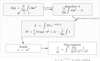
The $O(N)$ field appears quadratically after introducing the Lagrange multiplier $\lambda$. Integrating over the $N$ components gives an effective action $NW[\lambda]$, so the $N=\infty$ limit is controlled by a saddle point of $W$.

The saddle and the gap equation

The saddle equation is

$${\delta W\over\delta\lambda(x)}=0.$$

Using

$$\delta\operatorname{Tr}\log A=\operatorname{Tr}(A^{-1}\delta A),$$

with $A=-\partial^2+\lambda$, we find

$${1\over2}\langle x|{1\over -\partial^2+\lambda}|x\rangle -{1\over2g_0}=0.$$

Translation invariance suggests a constant saddle,

$$\lambda(x)=m^2.$$

Then the saddle equation becomes

$$\boxed{ {1\over g_0} =\int_{|p|<\Lambda}{d^2p\over(2\pi)^2}\,{1\over p^2+m^2}. }$$

This is the large-$N$ gap equation. The right-hand side is logarithmically divergent in two dimensions:

$$\int_{|p|<\Lambda}{d^2p\over(2\pi)^2}\,{1\over p^2+m^2} ={1\over4\pi}\log{\Lambda^2+m^2\over m^2}.$$

For $m\ll\Lambda$,

$${1\over g_0} ={1\over2\pi}\log{\Lambda\over m}+O(m^2/\Lambda^2).$$

Solving for $m$ gives

$$\boxed{ m=\Lambda\exp\left[-{2\pi\over g_0}\right] \left[1+O(m^2/\Lambda^2)\right]. }$$

This is the same dimensional transmutation scale found from the perturbative beta function in the large-$N$ limit.

This derivation used the infinite plane and a translation-invariant saddle. In a periodic box of side $L$, the same equation is instead

$${1\over g_0} ={1\over L^2}\sum_{p_\mu=2\pi n_\mu/L} {1\over p^2+m_L^2}.$$

The sum includes the constant mode $p=0$, whose contribution is $1/(L^2m_L^2)$. Consequently a finite box has a positive finite-size saddle $m_L$; one must not discard this zero mode and then interpret the result as spontaneous symmetry breaking. The integral formula and the scale $m$ are recovered when $Lm\gg1$.

Renormalized coupling and cutoff independence

The gap equation also shows how to remove the cutoff in practice. Define a running coupling at a subtraction scale $\mu$ by

$${1\over g(\mu)}={1\over g_0}-{1\over2\pi}\log{\Lambda\over\mu}.$$

Then the gap equation becomes

$${1\over g(\mu)}={1\over2\pi}\log{\mu\over m},$$

or

$$\boxed{m=\mu\exp\left[-{2\pi\over g(\mu)}\right].}$$

The cutoff $\Lambda$ has disappeared in favor of the measured coupling $g(\mu)$ and the physical mass $m$. This is the large-$N$ version of renormalization: the continuum limit is taken by tuning $g_0\to0$ as $\Lambda\to\infty$ while holding $m$ fixed.

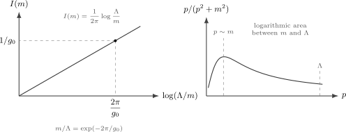
The gap equation is logarithmic in two dimensions: $1/g_0=(1/2\pi)\log(\Lambda/m)$ at weak coupling. A small dimensionless bare coupling is replaced by the exponentially small physical mass $m$.

The saddle value has a direct physical meaning. In the original action, $\lambda$ multiplies $\mathbf n^2$. At the saddle,

$${N\over2g_0}\int d^2x\,\lambda\mathbf n^2 \longrightarrow {N\over2g_0}\int d^2x\,m^2\mathbf n^2.$$

Thus the $N$ components of $\mathbf n$ acquire a mass $m$. The classical action had no mass scale, but the quantum theory has one.

Propagator and restoration of symmetry

At the saddle, the quadratic action is

$$S_{\rm quad} ={N\over2g_0}\int d^2x\, \mathbf n(-\partial^2+m^2)\mathbf n.$$

Therefore

$$\boxed{ \langle n^a(p)n^b(-p)\rangle ={g_0\over N}\,{\delta^{ab}\over p^2+m^2} +O(1/N^2). }$$

This normalization is consistent with the constraint. Indeed,

$$\langle\mathbf n^2(x)\rangle =\sum_{a=1}^N\langle n^a(x)n^a(x)\rangle =g_0\int^\Lambda {d^2p\over(2\pi)^2}{1\over p^2+m^2}=1,$$

where the last equality is exactly the gap equation.

After the $\mathbf n$ fields have been integrated out, this is how the constraint appears at leading order: the saddle enforces $\langle\mathbf n^2\rangle=1$. It does not mean that individual configurations of the resulting Gaussian saddle theory obey $\mathbf n^2(x)=1$ pointwise. Fluctuations of $\lambda$ restore the local constraint order by order in $1/N$.

It is often convenient to define a canonically normalized field

$$\Phi^a=\sqrt{N\over g_0}\,n^a.$$

Then

$$\langle\Phi^a(p)\Phi^b(-p)\rangle ={\delta^{ab}\over p^2+m^2}+O(1/N).$$

To test rather than assume symmetry restoration, allow a constant expectation value in one direction,

$$\langle n^1\rangle=v.$$

At leading order, the two saddle equations take the form

$$\boxed{ \begin{aligned} m^2v&=0,\\ v^2+g_0\int^\Lambda{d^2p\over(2\pi)^2}{1\over p^2+m^2}&=1. \end{aligned} }$$

There are two candidate branches. A symmetric branch has $v=0$ and $m>0$. An ordered branch would require $v\ne0$ and hence $m=0$. In two dimensions, however,

$$\int{d^2p\over(2\pi)^2}{1\over p^2}$$

diverges in the infrared. The ordered branch cannot satisfy the second saddle equation at nonzero $g_0$. The surviving infinite-volume saddle therefore has

$$v=0, \qquad m>0,$$

and the $O(N)$ symmetry is unbroken. At finite volume, $\langle n^a\rangle=0$ also follows from integrating the global orientation zero mode. The distinction between finite-volume averaging and genuine infrared restoration is developed on the next page.

The large-$N$ solution thus makes restoration concrete: the classical ordered direction is replaced by massive, degenerate $O(N)$ vector excitations.

The correlation length is

$$\xi={1\over m}.$$

At weak bare coupling, $m$ is exponentially small compared with the cutoff, so the model has a long scaling regime. This is why the perturbative RG was useful even though the true infrared theory is massive.

Why the saddle is nonperturbative

The mass gap

$$m=\Lambda e^{-2\pi/g_0}$$

has an essential singularity at $g_0=0$. Its Taylor expansion around $g_0=0$ vanishes term by term. This is why no finite order in ordinary perturbation theory can produce the mass gap.

Perturbation theory around a fixed classical direction gives massless transverse fields and logarithmic running. The large-$N$ saddle instead sums infinitely many diagrams before expanding. The infinite sum reorganizes the perturbation series so that the nonanalytic scale becomes visible.

One way to say this is that the large-$N$ saddle solves a self-consistency problem. The field is massive because $\lambda=m^2$, but $\lambda=m^2$ is chosen so that the massive fluctuations satisfy the constraint:

$$\langle\mathbf n^2\rangle=1.$$

The mass is not inserted by hand; it is the value of the collective field needed to make the quantum constraint true.

Fluctuations of the Lagrange multiplier

The next order in $1/N$ comes from fluctuations of $\lambda$ around its saddle value. Write schematically

$$\lambda(x)=m^2+\eta(x).$$

Expanding $W[\lambda]$ gives

$$W[m^2+\eta] =W[m^2]-{1\over4}\int {d^2q\over(2\pi)^2}\, \eta(q)\Pi(q)\eta(-q)+O(\eta^3),$$

where

$$\boxed{ \Pi(q)=\int {d^2k\over(2\pi)^2} {1\over(k^2+m^2)((k+q)^2+m^2)}. }$$

The minus sign is tied to the original $\lambda$ contour. After rotating to the steepest-descent fluctuation variable, the quadratic kernel is positive and the auxiliary-field propagator is proportional to $1/\Pi(q)$. The important physics is independent of this convention: the propagator of the collective field is the inverse of the bubble built from the massive $\mathbf n$ fields.

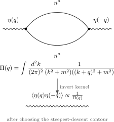
The quadratic action for the Lagrange-multiplier fluctuation is generated by a one-loop bubble of massive $\mathbf n$ fields. The collective-field propagator is proportional to $1/\Pi(q)$.

Using a Feynman parameter,

$$\Pi(q)=\int_0^1 dx\int {d^2\ell\over(2\pi)^2} {1\over[\ell^2+m^2+x(1-x)q^2]^2}.$$

The two-dimensional integral is finite:

$$\int {d^2\ell\over(2\pi)^2}{1\over(\ell^2+\Delta)^2} ={1\over4\pi\Delta}.$$

Thus

$$\Pi(q)={1\over4\pi}\int_0^1 dx\, {1\over m^2+x(1-x)q^2}.$$

For Euclidean $q^2>0$, this can be written as

$$\boxed{ \Pi(q) ={1\over \pi |q|\sqrt{q^2+4m^2}} \operatorname{artanh}\left({|q|\over\sqrt{q^2+4m^2}}\right). }$$

Two limits are especially useful. At small momentum,

$$\Pi(q)= {1\over4\pi m^2}+O(q^2/m^4).$$

At large Euclidean momentum,

$$\Pi(q)= {1\over2\pi q^2}\log{q^2\over m^2} +O\left({m^2\over q^4}\log{q^2\over m^2}\right).$$

The large-momentum logarithm is the same logarithm that appeared in the perturbative RG. In the large-$N$ solution, it sits inside the propagator of the collective field.

1/N counting

The $1/N$ expansion becomes transparent after rescaling to a canonically normalized $O(N)$ vector field,

$$n^a=\sqrt{g_0\over N}\,\Phi^a.$$

The action is

$$S={1\over2}\int d^2x\,\Phi^a(-\partial^2+\lambda)\Phi^a -{N\over2g_0}\int d^2x\,\lambda.$$

Expanding around the saddle and rotating to the stable fluctuation variable, one may write schematically

$$\lambda=m^2+{i\over\sqrt N}\chi.$$

The factor $1/\sqrt N$ gives $\chi$ an order-one propagator. The factor of $i$ records the local steepest-descent direction; changing the original multiplier convention can move this factor between the contour and the vertices.

Then

$$S={1\over2}\int d^2x\,\Phi^a(-\partial^2+m^2)\Phi^a +{i\over2\sqrt N}\int d^2x\,\chi\Phi^a\Phi^a+\text{terms depending only on }\chi.$$

The rules are therefore:

$$\Phi\text{ propagator}\sim O(1), \qquad \chi\Phi\Phi\text{ vertex}\sim O(N^{-1/2}), \qquad \text{closed }\Phi\text{ loop}\sim O(N).$$

A bubble with two $\chi\Phi\Phi$ vertices is $O(1)$, because the factor $N$ from summing the internal $O(N)$ index cancels the two factors of $N^{-1/2}$. This is why the bubble must be kept in the leading auxiliary-field propagator.

This is a saddle expansion in the number of components, not a power series in $g_0$. It can therefore contain the leading mass $m\sim e^{-2\pi/g_0}$ even though that scale is nonperturbative in the ordinary coupling.

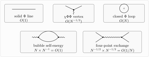
In canonical variables, the $\chi\Phi\Phi$ vertex carries $N^{-1/2}$, while each closed $\Phi$ loop carries $N$. The bubble correction to the $\chi$ propagator is therefore order one, and four-point scattering through $\chi$ exchange is order $1/N$.

For example, the connected four-point function of the normalized $\Phi$ fields begins at order $1/N$. Its index structure is fixed by $O(N)$ symmetry:

$$\Gamma^{(4)}_{abcd}(p_i) ={1\over N}\left[ \delta_{ab}\delta_{cd}\,\mathcal A(s) +\delta_{ac}\delta_{bd}\,\mathcal A(t) +\delta_{ad}\delta_{bc}\,\mathcal A(u) \right] +O(N^{-2}),$$

where $s,t,u$ denote the three momentum channels after analytic continuation, and $\mathcal A$ is proportional to the inverse bubble $1/\Pi$. Overall signs and factors of $2$ depend on the precise normalization of the auxiliary fluctuation, but the $1/N$ scaling and the channel structure are invariant statements.

At high Euclidean momentum, the inverse bubble behaves as

$${1\over\Pi(q)}\sim {2\pi q^2\over \log(q^2/m^2)}.$$

The logarithm in the denominator is the large-$N$ version of asymptotic freedom. Interactions become weaker at short distances, but only logarithmically.

The effective action as a diagrammatic resummation

The saddle calculation can be rephrased in ordinary diagrams. The Lagrange multiplier couples to $\mathbf n^2$. Integrating out $\mathbf n$ produces a determinant,

$${N\over2}\operatorname{Tr}\log(-\partial^2+\lambda),$$

which is the sum of closed $\mathbf n$ loops with any number of external $\lambda$ insertions:

$$\operatorname{Tr}\log(A+\eta) =\operatorname{Tr}\log A +\operatorname{Tr}(A^{-1}\eta) -{1\over2}\operatorname{Tr}(A^{-1}\eta A^{-1}\eta) +\cdots.$$

The linear term vanishes at the saddle because it is exactly the gap equation. The quadratic term is the bubble $\Pi(q)$. Higher terms give cubic and higher self-interactions of the collective field, suppressed by powers of $1/\sqrt N$ after the canonical rescaling.

This is a good example of what “large $N$ solves the theory” really means. It does not mean that every diagram disappears. It means that a special infinite class of diagrams is promoted to the leading approximation and summed into a new propagator. The expansion then proceeds around the self-consistent massive theory, not around the massless classical one.

Relation to the perturbative beta function

The large-$N$ gap equation can be written as

$${1\over g(\mu)}={1\over g_0}-{1\over2\pi}\log{\Lambda\over\mu},$$

so that

$$\mu{dg\over d\mu}=-{g^2\over2\pi}+O(1/N).$$

This is precisely the large-$N$ limit of the perturbative result for the $O(N)$ model. The scale where $g(\mu)$ becomes order one is

$$\mu\sim \Lambda e^{-2\pi/g_0},$$

which matches the saddle-point mass $m$.

The important conceptual improvement is that the large-$N$ computation continues past the point where perturbation theory around the massless fields fails. It gives a massive propagator and a systematic expansion in $1/N$. The running coupling warned us that a scale must appear; the saddle shows how it appears.

A strong-coupling check from the lattice

The weak-coupling large-$N$ saddle gives $m\ll\Lambda$. The opposite limit is also useful as a sanity check. Put the two-dimensional Euclidean model on a spatial lattice and interpret one direction as imaginary time. The Hamiltonian of a chain of rotors has the schematic form

$$H={1\over2}\sum_x\left(g_0 L_x^2+{1\over g_0}(\mathbf n_x-\mathbf n_{x+1})^2\right),$$

where $L_x^2$ is the Laplacian on $S^{N-1}$ at site $x$. At very strong coupling, $g_0\to\infty$, the sites decouple and the ground state at each site is the rotational singlet,

$$\ell_x=0.$$

The first excitation has angular momentum $\ell_x=1$ and costs an energy of order $g_0$. Thus the strong-coupling model is also gapped. The weak-coupling and strong-coupling descriptions produce the gap in very different ways, but they agree on the qualitative point: in the two-dimensional $O(N)$ model with $N>2$, there is no ordinary Goldstone phase.

This lattice picture is also a bridge to the next topic. Spin chains and antiferromagnets can be described by sigma models, but the topological term changes the infrared physics in a way that the ordinary large-$N$ saddle does not capture.

Summary

The large-$N$ limit of the two-dimensional $O(N)$ nonlinear sigma model is controlled by a Lagrange-multiplier saddle. With

$$S={N\over2g_0}\int d^2x\,(\partial\mathbf n)^2, \qquad \mathbf n^2=1,$$

introducing $\lambda$ and integrating over the $N$ components of $\mathbf n$ gives

$$Z=\int\mathcal D\lambda\,e^{-NW[\lambda]}, \qquad W[\lambda]={1\over2}\operatorname{Tr}\log(-\partial^2+\lambda)-{1\over2g_0}\int\lambda.$$

The constant saddle $\lambda=m^2$ obeys

$${1\over g_0}=\int^\Lambda {d^2p\over(2\pi)^2}{1\over p^2+m^2},$$

so

$$m=\Lambda e^{-2\pi/g_0}$$

at weak coupling. The propagator is massive,

$$\langle n^a(p)n^b(-p)\rangle={g_0\over N}{\delta^{ab}\over p^2+m^2},$$

and $O(N)$ remains unbroken. Fluctuations of $\lambda$ are governed by the bubble

$$\Pi(q)=\int {d^2k\over(2\pi)^2} {1\over(k^2+m^2)((k+q)^2+m^2)},$$

so the collective-field propagator is proportional to $1/\Pi(q)$. The resulting $1/N$ expansion is a controlled expansion around a dynamically massive theory.

Common pitfalls

Forgetting the large-N scaling of the coupling. The useful limit keeps $g_0=N\alpha_0$ fixed. Holding $\alpha_0$ fixed as $N\to\infty$ sends the theory to a different, strongly scaled problem.

Confusing $\lambda$ with the mass rather than the mass squared. In the action, $\lambda$ appears as $p^2+\lambda$. The constant saddle is $\lambda=m^2$.

Treating the Lagrange-multiplier contour as a harmless real integral. The constraint is imposed by a contour integral. Around the saddle one often rotates the fluctuation variable to the steepest-descent direction. This can flip signs in intermediate formulas for the $\lambda$ propagator.

Dropping the finite-volume zero mode. On a torus the momentum integral becomes a discrete sum that includes $p=0$. Omitting that term can manufacture a false ordered saddle and confuse finite-volume symmetry averaging with spontaneous symmetry breaking.

Expecting Goldstone bosons because the classical field lives on a sphere. The two-dimensional quantum theory has no ordinary long-range ordered direction. In the large-$N$ solution the infrared divergence excludes the massless ordered branch and leaves the symmetric massive saddle.

Thinking that large N is merely one-loop perturbation theory. The determinant is a one-loop functional of $\lambda$, but it sums infinitely many diagrams in the original coupling and produces the nonperturbative scale $m\sim e^{-2\pi/g_0}$.

Exercises

Exercise 1: solving the large-N gap equation

Evaluate

$$I(m,\Lambda)=\int_{|p|<\Lambda}{d^2p\over(2\pi)^2}{1\over p^2+m^2}$$

and use $I(m,\Lambda)=1/g_0$ to find $m$ for $m\ll\Lambda$.

Solution

In polar coordinates,

$$d^2p=p\,dp\,d\theta.$$

Therefore

$$I(m,\Lambda) ={1\over(2\pi)^2}\int_0^{2\pi}d\theta\int_0^\Lambda {p\,dp\over p^2+m^2} ={1\over2\pi}\int_0^\Lambda {p\,dp\over p^2+m^2}.$$

The remaining integral is

$$\int_0^\Lambda {p\,dp\over p^2+m^2} ={1\over2}\log{\Lambda^2+m^2\over m^2}.$$

Thus

$$I(m,\Lambda)={1\over4\pi}\log{\Lambda^2+m^2\over m^2}.$$

For $m\ll\Lambda$,

$$I(m,\Lambda)={1\over2\pi}\log{\Lambda\over m}+O(m^2/\Lambda^2).$$

The gap equation $I=1/g_0$ gives

$${1\over g_0}={1\over2\pi}\log{\Lambda\over m},$$

so

$$m=\Lambda e^{-2\pi/g_0}.$$

Exercise 2: checking the constraint

Using

$$\langle n^a(p)n^b(-p)\rangle ={g_0\over N}{\delta^{ab}\over p^2+m^2},$$

show that $\langle\mathbf n^2(x)\rangle=1$ at leading order in $1/N$.

Solution

At coincident points,

$$\langle n^a(x)n^b(x)\rangle ={g_0\over N}\delta^{ab} \int^\Lambda {d^2p\over(2\pi)^2}{1\over p^2+m^2}.$$

Sum over $a=b$:

$$\langle\mathbf n^2(x)\rangle =\sum_{a=1}^N\langle n^a(x)n^a(x)\rangle =g_0\int^\Lambda {d^2p\over(2\pi)^2}{1\over p^2+m^2}.$$

The gap equation says

$$\int^\Lambda {d^2p\over(2\pi)^2}{1\over p^2+m^2}={1\over g_0}.$$

Therefore

$$\langle\mathbf n^2(x)\rangle=1.$$

Exercise 3: the bubble integral

Show that

$$\Pi(q)=\int {d^2k\over(2\pi)^2} {1\over(k^2+m^2)((k+q)^2+m^2)}$$

can be written as

$$\Pi(q)={1\over4\pi}\int_0^1 dx\,{1\over m^2+x(1-x)q^2}.$$

Then derive the small-$q$ limit $\Pi(0)=1/(4\pi m^2)$.

Solution

Use the Feynman-parameter identity

$${1\over AB}=\int_0^1 dx\,{1\over[xA+(1-x)B]^2}.$$

With

$$A=k^2+m^2, \qquad B=(k+q)^2+m^2,$$

we obtain

$$xA+(1-x)B=(k+(1-x)q)^2+m^2+x(1-x)q^2.$$

After shifting the loop momentum to $\ell=k+(1-x)q$,

$$\Pi(q)=\int_0^1 dx\int {d^2\ell\over(2\pi)^2} {1\over[\ell^2+m^2+x(1-x)q^2]^2}.$$

In two dimensions,

$$\int {d^2\ell\over(2\pi)^2}{1\over(\ell^2+\Delta)^2} ={1\over4\pi\Delta}.$$

Therefore

$$\Pi(q)={1\over4\pi}\int_0^1 dx\,{1\over m^2+x(1-x)q^2}.$$

At $q=0$ this gives

$$\Pi(0)={1\over4\pi}\int_0^1 {dx\over m^2} ={1\over4\pi m^2}.$$

Exercise 4: leading 1/N scaling of the four-point function

In canonical variables, the $\chi\Phi\Phi$ vertex scales as $N^{-1/2}$ and the $\chi$ propagator is order $N^0$. What is the large-$N$ order of the four-point connected diagram made from one $\chi$ exchange between two pairs of $\Phi$ fields?

Solution

The exchange diagram has two $\chi\Phi\Phi$ vertices and one $\chi$ propagator. Each vertex contributes a factor

$$N^{-1/2}.$$

The $\chi$ propagator is order one:

$$N^0.$$

Therefore the total scaling is

$$N^{-1/2}\times N^0\times N^{-1/2}=N^{-1}.$$

Thus the connected four-point function of normalized $\Phi$ fields begins at order $1/N$. This agrees with the physical picture that the $N=\infty$ theory is a free massive vector theory, and interactions first appear at the next order.

Exercise 5: matching the large-N beta function

Starting from the one-loop sigma-model beta function

$$\mu{d\alpha\over d\mu}=-{N-2\over2\pi}\alpha^2+O(\alpha^3),$$

set $g=N\alpha$ and take $N\to\infty$ with $g$ fixed. Derive the leading beta function for $g$ and compare its generated scale with the large-$N$ saddle mass.

Solution

Since $g=N\alpha$,

$$\mu{dg\over d\mu}=N\mu{d\alpha\over d\mu}.$$

Substitute the beta function:

$$\mu{dg\over d\mu} =-N{N-2\over2\pi}\alpha^2+O(N\alpha^3).$$

Using $\alpha=g/N$,

$$\mu{dg\over d\mu} =-{N-2\over N}{g^2\over2\pi}+O(g^3/N^2).$$

At leading large $N$,

$$\mu{dg\over d\mu}=-{g^2\over2\pi}+O(1/N).$$

Solving this equation gives

$${1\over g(\mu)}={1\over g_0}+{1\over2\pi}\log{\mu\over\Lambda}.$$

The coupling becomes order one at

$$\mu\sim\Lambda e^{-2\pi/g_0}.$$

This is the same exponential scale as the saddle-point mass

$$m=\Lambda e^{-2\pi/g_0}.$$

Exercise 6: the finite-volume zero mode

On a periodic square of side $L$, the large-$N$ gap equation is

$${1\over g_0}={1\over L^2}\sum_p{1\over p^2+m_L^2}.$$

Use only the $p=0$ term to prove that $m_L^2\ge g_0/L^2$. What does this inequality say about a putative massless saddle at finite $L$?

Solution

Every term in the Euclidean momentum sum is nonnegative. Keeping only the constant mode therefore gives

$${1\over g_0} ={1\over L^2}\sum_p{1\over p^2+m_L^2} \ge {1\over L^2m_L^2}.$$

Multiplying by $g_0L^2m_L^2$ yields

$$m_L^2\ge {g_0\over L^2}.$$

Thus the finite-volume saddle cannot be massless. This bound tends to zero as $L\to\infty$, so it does not by itself determine the infinite-volume gap; the full sum is needed to recover $m=\Lambda e^{-2\pi/g_0}$.

References

• E. Brézin and J. Zinn-Justin, “Spontaneous Breakdown of Continuous Symmetries Near Two Dimensions,” Physical Review B 14 (1976) 3110–3120, doi:10.1103/PhysRevB.14.3110.
• S. Coleman, “There Are No Goldstone Bosons in Two Dimensions,” Communications in Mathematical Physics 31 (1973) 259–264, doi:10.1007/BF01646487.
• M. Moshe and J. Zinn-Justin, “Quantum Field Theory in the Large $N$ Limit: A Review,” Physics Reports 385 (2003) 69–228, doi:10.1016/S0370-1573(03)00263-1.

Further reading

• A. M. Polyakov, Gauge Fields and Strings, Contemporary Concepts in Physics, Vol. 3, Harwood Academic Publishers, Chur, 1987.
• A. Zee, Quantum Field Theory in a Nutshell, 2nd ed., Princeton University Press, Princeton, 2010.
• J. Zinn-Justin, Quantum Field Theory and Critical Phenomena, 5th ed., Oxford University Press, Oxford, 2021.