Stress-Tensor OPE and Conformal Ward Identities

The stress tensor generates a conformal transformation by a contour integral around the field being transformed. This lesson derives that statement from local Ward contacts, explains when those contacts determine a complete correlation function on the plane, and uses the result to distinguish primaries from their derivative descendants. We work in a two-dimensional Euclidean CFT with an improved stress tensor and ordinary primary fields of definite weights. Global vacuum assumptions will be stated when they are needed.

Required background. Stress tensors and current Ward identities supply metric variation, insertion contacts and the normalization of the chiral stress tensor. Finite conformal maps supply the local primary-field transformation law.

Holomorphic stress tensors and local primary fields

Let $\mathcal T_{ab}$ denote the Euclidean metric stress tensor defined by the plus covariant-metric variation $\delta S_E=\tfrac12\int d^2x\,\sqrt g\,\mathcal T^{ab}\delta g_{ab}$. In a flat complex chart $z=x^1+ix^2$, with $d^2z=dx^1dx^2$, the residue-normalized components are

$$T=2\pi\mathcal T_{zz},\qquad \bar T=2\pi\mathcal T_{\bar z\bar z},\qquad \Theta=2\pi\mathcal T_{z\bar z}.$$

Conservation gives

$$\bar\partial T+\partial\Theta=0,\qquad \partial\bar T+\bar\partial\Theta=0.$$

At the conformal fixed point, choose the improvement so that $\Theta=0$ at separated points on the flat plane. We assume the appropriate conserved stress tensor exists; scale invariance alone is not being used as a general proof of conformal invariance. Consequently,

$$\bar\partial T=0,\qquad \partial\bar T=0$$

away from insertions. Contact terms remain at insertions, and background curvature can introduce trace anomalies.

For a primary $O$ of weights $(h,\bar h)$, use the course’s positive active pullback,

$$O(z,\bar z)\longmapsto [f'(z)]^h[\bar f'(\bar z)]^{\bar h} O(f(z),\bar f(\bar z)).$$

This is a local statement on a nonsingular chart with $f'\ne0$ and a consistent branch for noninteger powers. A globally implemented map additionally requires the appropriate domain, state and spin structure. The two weights give dimension $\Delta=h+\bar h$ and spin $s=h-\bar h$. For $f(z)=z+\epsilon(z)$, the holomorphic variation is

$$\delta_\epsilon O =\epsilon\partial O+h(\partial\epsilon)O.$$

The antiholomorphic contribution is $\bar\epsilon\bar\partial O+\bar h(\bar\partial\bar\epsilon)O$. Below the holomorphic and antiholomorphic variations may be treated independently and then combined.

Local Ward contacts with a fixed action sign

A holomorphic transformation has $\bar\partial\epsilon=0$. To derive its local Ward identity, extend its parameter smoothly away from the insertions. Choose the extension to agree with a holomorphic function near each insertion and to have compact support. It need not be holomorphic where the cutoff changes.

For the active matter transformation, combined with the local frame rotation and Weyl transformation that restore the conformal frame near the insertions, the stress insertion has the normalization

$$\delta S_E=-\frac1\pi\int d^2z\, \left[T\,\bar\partial\epsilon +\bar T\,\partial\bar\epsilon\right].$$

The sign follows from the metric definition, rather than from a choice of notation for the path-integral weight. At fixed flat metric, the active matter/frame variation is minus the metric pullback. The symmetric improved metric stress includes the spin contribution. Its traceless contraction is

$$-\int d^2z\,\mathcal T^{ab}\partial_a\epsilon_b =-2\int d^2z\, \left[\mathcal T_{zz}\bar\partial\epsilon +\mathcal T_{\bar z\bar z}\partial\bar\epsilon\right],$$

which yields the displayed $-1/\pi$ coefficient. The trace and spin contacts are handled by the Weyl and local-frame Ward identities; a scalar coordinate pullback alone would not supply the spin contact of a spinful field. This step assumes a compatible regulator and renormalized operators; anomalous background terms must be included when present. It does not assign the primary transformation law to an arbitrary nonconformal diffeomorphism.

The combined metric, frame and Weyl derivation is given in Di Francesco, Mathieu and Sénéchal 1997, § 5.2.3, pp. 123–126, Eqs. 5.54–5.69. Their covariant-metric tensor and infinitesimal field parameter both have the opposite signs to ours; the residue-normalized $T$ and its OPE coefficients agree after these translations.

Let $X=\prod_{k=1}^n O_k(z_k,\bar z_k)$ have distinct insertion points, and write $G=\langle X\rangle$. With the Euclidean weight, the normalized change-of-variables identity in this flat vacuum is

$$0=\langle\delta X\rangle-\langle X\delta S_E\rangle.$$

More generally the second term is connected to $X$; the vacuum stress variation vanishes here. Considering the holomorphic part and integrating by parts gives

$$0=\sum_k\left[ \epsilon(z_k)\partial_{z_k} +h_k(\partial\epsilon)(z_k) \right]G -\frac1\pi\int d^2z\, \epsilon(z)\bar\partial_z\langle T(z)X\rangle.$$

The metric, local-frame and Weyl Ward identities fix the contact prescription used here. In that prescription the holomorphic contact equation is

$$\bar\partial_z\langle T(z)X\rangle =\pi\sum_k\left[ -h_k\,\partial_z\delta^{(2)}(z-z_k) +\delta^{(2)}(z-z_k)\partial_{z_k} \right]G.$$

The derivative of the delta acts on the test function with a minus sign, producing $+h_k\partial\epsilon(z_k)$. This checks the relative signs without guessing the OPE. The cutoff tests alone probe only holomorphic jets near the insertions: they would not detect an additional $\bar\partial\delta^{(2)}$ contact. The background Ward prescription, rather than those restricted tests alone, fixes this freedom. For theories without a Lagrangian path integral, the same equation is the local stress-tensor Ward identity; the contour argument below uses that identity directly.

Distributional poles and their local operator products

The locally integrable distribution $1/z$ satisfies

$$\bar\partial\frac1z=\pi\delta^{(2)}(z).$$

Indeed, for a smooth compactly supported test function $u$,

$$-\int d^2z\,\frac1z\,\bar\partial u =\pi u(0),$$

as follows by excising a small disk and applying Cauchy–Green. The factor $\pi$ uses the Cartesian area element and counterclockwise positive circles.

The higher powers $1/z^{m+1}$, $m\ge1$, are not locally integrable as ordinary functions. In this Ward identity define their extension by derivatives:

$$\left[\frac1{z^{m+1}}\right]_{\rm dist} =\frac{(-1)^m}{m!}\,\partial^m\frac1z.$$

It follows that

$$\bar\partial \left[\frac1{z^{m+1}}\right]_{\rm dist} =\frac{\pi(-1)^m}{m!}\, \partial^m\delta^{(2)}(z).$$

In particular, the double pole gives a negative derivative-delta contact. These are specified distributional extensions; changing a contact prescription requires checking the corresponding Ward identity, not just comparing functions at noncoincident points.

The contact equation therefore fixes the principal parts of the stress insertion:

$$\langle T(z)X\rangle =\sum_k\left[ \frac{h_k}{(z-z_k)^2} +\frac1{z-z_k}\partial_{z_k} \right]G+H(z).$$

Here $H$ is holomorphic in the region being considered. Local contacts alone do not set $H$ to zero. A state, boundary or global geometry can supply additional regular data. We will eliminate $H$ for the sphere vacuum below. The contact construction and its regular remainder appear in Di Francesco, Mathieu and Sénéchal 1997, § 5.2.1, pp. 118–120, Eqs. 5.32–5.41.

Taking the local singular part gives the primary OPE,

$$T(z)O(w,\bar w) \sim \frac{h\,O(w,\bar w)}{(z-w)^2} +\frac{\partial_w O(w,\bar w)}{z-w}.$$

The double pole gives the local dilation/rotation weight; the simple pole moves the insertion. Neither term creates an independent primary of a new weight. The antiholomorphic OPE has $\bar h$, $\partial_{\bar w}$ and $\bar z-\bar w$ in the corresponding places. See Di Francesco, Mathieu and Sénéchal 1997, § 5.3, p. 127, Eqs. 5.71–5.72 for the stress OPE inside correlators.

Contours as local conformal generators

Let $C_w$ go once counterclockwise around $w$ and no other insertion. If $\epsilon_0$ is holomorphic inside $C_w$, its expansion at $w$ gives

$$\frac1{2\pi i}\oint_{C_w}dz\, \epsilon_0(z)T(z)O(w,\bar w) =\epsilon_0(w)\partial_w O +h\,\epsilon_0'(w)O.$$

Only the linear term of $\epsilon_0$ multiplies the double pole into a residue. The constant term multiplies the simple pole. Thus this contour operation is exactly $\delta_{\epsilon_0}O$ in the positive active convention.

The same operation can be obtained from the smooth cutoff used in the Ward derivation. Take $\epsilon=\chi\epsilon_0$, with $\chi=1$ near $w$ and $\chi=0$ outside a larger disk containing no other insertion. Then $\bar\partial\chi$ is supported in the intervening annulus. For $F(z)=\epsilon_0(z)\langle T(z)X\rangle$, Cauchy–Green on that annulus gives

$$\int d^2z\,(\bar\partial\chi)F(z) =-\frac1{2i}\oint_{C_w}F(z)\,dz.$$

Combining this with the action coefficient yields

$$-\frac1\pi\int d^2z\,(\bar\partial\chi)F(z) =\frac1{2\pi i}\oint_{C_w}F(z)\,dz.$$

The annulus is the support of the smooth variation; the point $w$ is the support of the contact distribution after integration by parts. There is no nonzero globally holomorphic compactly supported parameter.

Now let $C$ surround several separated insertions, and let $C_k$ be disjoint small counterclockwise circles around them. Require $F$ to be single-valued and holomorphic on the punctured region swept out in deforming the contours, with no additional cuts, singularities or boundaries. The boundary of that region is $C-\sum_k C_k$, so

$$\frac1{2\pi i}\oint_C dz\, \epsilon_0(z)\langle T(z)X\rangle =\sum_k\left[ \epsilon_0(z_k)\partial_{z_k} +h_k\epsilon_0'(z_k) \right]G.$$

In the figure, distinguish the shaded annular support from the insertion point in the upper panel. The lower panel shows why the local contours on the right-hand side all retain counterclockwise orientation.

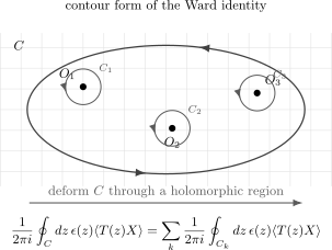
A smooth cutoff localizes the variation to an annulus, while integration by parts gives contacts at the enclosed insertion. On a punctured planar domain with no other singularities, cuts or boundary contributions, a counterclockwise contour equals the sum of the counterclockwise local contours. The diagram is schematic; it does not assert that an arbitrary outer contour integral vanishes.

Contour identities on other surfaces remain useful, but their additional cycles, boundaries and monodromies require explicit data. The planar deformation above cannot silently discard those contributions.

The plane vacuum and global conformal constraints

Assume now the globally conformally invariant plane vacuum, equivalently the sphere with no insertion at infinity. The stress tensor has a Schwarzian term under a general map,

$$T(z)\longmapsto [f'(z)]^2T(f(z))+\frac{c}{12}\{f,z\}, \qquad \{f,z\}=\frac{f'''}{f'}-\frac32\left(\frac{f''}{f'}\right)^2.$$

Here $c$ is the holomorphic central charge. Its derivation belongs to the stress self-OPE; the finite law and the relevant Schwarzian properties are stated in Di Francesco, Mathieu and Sénéchal 1997, § 5.4.1, pp. 136–137, Eqs. 5.123–5.133. For the present argument, only the Möbius inversion $w=1/z$ is needed: its Schwarzian vanishes. Since $dw/dz=-z^{-2}$, regularity at $w=0$ implies

$$\langle T(z)X\rangle=O(z^{-4}) \qquad (z\to\infty).$$

Thus $T$ transforms as a quadratic differential between these two Möbius charts, even though it does not do so under a general conformal map. This is the infinity argument of Di Francesco, Mathieu and Sénéchal 1997, § 5.2.2, p. 123, Eq. 5.52. The sentence preceding that equation contains a weight typo: holomorphic $T$ has $(h,\bar h)=(2,0)$, and $\bar T$ has $(0,2)$.

The rational principal-part expression decays at least as $1/z$. Consequently the difference $H$ is an entire function that tends to zero at infinity. Liouville’s theorem sets it to zero. We obtain the full plane-vacuum Ward identity

$$\boxed{ \langle T(z)X\rangle =\sum_k\left[ \frac{h_k}{(z-z_k)^2} +\frac1{z-z_k}\partial_{z_k} \right]G. }$$

Its antiholomorphic version follows in the same way. This uniqueness argument uses the global vacuum condition; it is stronger than the local contact equation.

The globally regular holomorphic vector fields on the sphere are $\epsilon(z)=a_{-1}+a_0z+a_1z^2$. For these parameters, the large contour integral vanishes because of the $z^{-4}$ falloff. Equivalently, expanding the plane Ward identity at large $z$ gives

$$\begin{aligned} \langle T(z)X\rangle ={}&\frac1z\sum_k\partial_{z_k}G\\ &+\frac1{z^2}\sum_k(z_k\partial_{z_k}+h_k)G\\ &+\frac1{z^3}\sum_k(z_k^2\partial_{z_k}+2h_kz_k)G +O(z^{-4}). \end{aligned}$$

The first three coefficients must vanish:

Parameter	Transformation	Constraint on $G$
$1$	Translation	$\sum_k\partial_{z_k}G=0$
$z$	Dilation and rotation	$\sum_k(z_k\partial_{z_k}+h_k)G=0$
$z^2$	Special conformal transformation	$\sum_k(z_k^2\partial_{z_k}+2h_kz_k)G=0$

There are three corresponding antiholomorphic equations. Their derivation does not require unitarity, but it does require the specified vacuum and transformation laws. The contour and global constraints are developed in Di Francesco, Mathieu and Sénéchal 1997, § 5.2.2, pp. 121–123, Eqs. 5.42–5.53.

A stress insertion in a two-point function

For ordinary primaries with diagonalizable weights, the global constraints give a nonzero two-point function only when the two fields have equal holomorphic and equal antiholomorphic weights. On a fixed branch at separated points,

$$G_{12}= \frac{C_{12}}{z_{12}^{2h}\bar z_{12}^{2\bar h}}, \qquad z_{12}=z_1-z_2.$$

Exercise 2 derives the equal-weight condition. The constant $C_{12}$ is a bilinear pairing in the space of fields with those weights; the Ward identities do not determine it. Logarithmic representations require a different argument because their scaling operators need not be diagonalizable.

The single-stress Ward identity gives a useful additional check. Since $\partial_{z_1}G_{12}=-2hG_{12}/z_{12}$ and $\partial_{z_2}G_{12}=+2hG_{12}/z_{12}$,

$$\begin{aligned} \frac{\langle T(z)O_1O_2\rangle}{G_{12}} ={}&\frac{h}{(z-z_1)^2} +\frac{h}{(z-z_2)^2}\\ &-\frac{2h}{z_{12}} \left[\frac1{z-z_1}-\frac1{z-z_2}\right]\\ ={}&\frac{h\,z_{12}^2} {(z-z_1)^2(z-z_2)^2}, \end{aligned}$$

when $G_{12}\ne0$. Near either insertion this has the required double and simple poles. At infinity it decays as $z^{-4}$. The local OPE and the global vacuum condition are both visible in one correlator.

Derivative descendants and quasiprimary fields

If $O$ is primary, then $V=\partial O$ has weights $(h+1,\bar h)$. Differentiate its variation at fixed coordinates:

$$\begin{aligned} \delta_\epsilon(\partial O) &=\partial\left[\epsilon\partial O+h(\partial\epsilon)O\right]\\ &=\epsilon\partial^2O+(h+1)(\partial\epsilon)\partial O +h(\partial^2\epsilon)O. \end{aligned}$$

The first two terms are those of a primary of weight $h+1$. The last term mixes in $O$. Differentiating the OPE displays the same effect:

$$T(z)\partial O(w) \sim \frac{2h\,O(w)}{(z-w)^3} +\frac{(h+1)\partial O(w)}{(z-w)^2} +\frac{\partial^2O(w)}{z-w}.$$

The cubic pole contributes $(2h)(\epsilon''/2)O=h\epsilon''O$ to the residue. A shifted scaling weight by itself therefore does not make a derivative primary. If $h=0$, this obstruction vanishes algebraically; in a positive radial inner product, the level-one descendant of a weight-zero primary is null. A nonzero representative or a logarithmic theory requires its own representation assumptions.

A primary has this covariant law for arbitrary local holomorphic parameters. A quasiprimary has it only for the global generators $1,z,z^2$ and their antiholomorphic partners. A descendant is obtained by negative stress-tensor modes; the first is $\partial O=L_{-1}O$. A descendant can be quasiprimary after appropriate linear combinations, even when it is not primary. These are local representation statements; a global group action on fields with spin may require a covering group. The distinction and the derivative example are discussed in Di Francesco, Mathieu and Sénéchal 1997, § 5.1.4, p. 116, Eqs. 5.21–5.23.

To see the distinction at the origin, define

$$L_n=\frac1{2\pi i}\oint_0dz\,z^{n+1}T(z).$$

The action on a local field is understood through radial ordering: the difference of contours outside and inside the insertion shrinks to its local residue. For a primary,

$$\begin{gathered} [L_{-1},O(0)]=\partial O(0),\qquad [L_0,O(0)]=hO(0),\\ [L_n,O(0)]=0\quad(n>0). \end{gathered}$$

With definite weight, the $n=1$ condition is the holomorphic quasiprimary condition; all positive modes characterize a primary. The corresponding statements for states also require the radial vacuum and the state–operator map.

The stress tensor itself is quasiprimary. For nonzero central charge its Schwarzian term prevents it from being an ordinary primary under all local maps. The Virasoro algebra and stress tensor develops its self-OPE and modes. Its field-variation convention uses the opposite parameter, $\epsilon_{\rm ref}=-\epsilon$; the stress OPE and Laurent-mode normalization agree.

Common pitfalls

Dropping insertion contacts. Holomorphicity means $\bar\partial T=0$ at separated points. Its distributional contact terms are precisely what generate the conformal variation of inserted fields.

Assuming poles determine every state. The local Ward equation leaves a regular holomorphic term. Setting it to zero needs the global vacuum and infinity assumptions used above.

Reversing the small contours. Inner boundaries of a punctured domain are clockwise. After moving them to the other side of the contour equation, the local contours are counterclockwise and their residues enter with a plus sign.

Calling every derivative primary. Check the entire stress OPE, including higher poles. Scaling weight alone does not control the inhomogeneous terms of a local transformation.

Exercises

Exercise 1: Extracting the conformal variation

Use the OPE

$$T(z)O(w)\sim {hO(w)\over(z-w)^2}+{\partial O(w)\over z-w}$$

to show the following identity. Take a counterclockwise contour around only $w$ and let $\epsilon$ be holomorphic on its disk.

$${1\over2\pi i}\oint_w dz\,\epsilon(z)T(z)O(w) = \epsilon(w)\partial O(w)+h(\partial\epsilon)(w)O(w).$$

Solution

Expand $\epsilon(z)$ around $w$:

$$\epsilon(z)=\epsilon(w)+(z-w)\partial\epsilon(w)+{1\over2}(z-w)^2\partial^2\epsilon(w)+\cdots.$$

Then

$$\epsilon(z)T(z)O(w) \sim \epsilon(z){hO(w)\over(z-w)^2} + \epsilon(z){\partial O(w)\over z-w}.$$

Only the coefficient of $(z-w)^{-1}$ contributes to the contour integral. From the double-pole term, the residue is

$$h(\partial\epsilon)(w)O(w).$$

From the simple-pole term, the residue is

$$\epsilon(w)\partial O(w).$$

Therefore

$${1\over2\pi i}\oint_w dz\,\epsilon(z)T(z)O(w) = \epsilon(w)\partial O(w)+h(\partial\epsilon)(w)O(w).$$

Exercise 2: Two-point functions from global Ward identities

In the globally invariant plane vacuum, with separated insertions and a fixed branch, let $G(z_1,z_2)=\langle O_1(z_1)O_2(z_2)\rangle$ be a holomorphic two-point function of primary fields with weights $h_1$ and $h_2$. Use the three global Ward identities to show that $G$ can be nonzero only if $h_1=h_2$, and then

$$G(z_1,z_2)={C_{12}\over (z_1-z_2)^{2h_1}}.$$

Solution

The translation Ward identity gives

$$(\partial_{z_1}+\partial_{z_2})G=0,$$

so $G$ depends only on $z_{12}=z_1-z_2$:

$$G(z_1,z_2)=F(z_{12}).$$

The dilation Ward identity gives

$$\left(z_1\partial_{z_1}+z_2\partial_{z_2}+h_1+h_2\right)G=0.$$

Since

$$z_1\partial_{z_1}+z_2\partial_{z_2}=z_{12}{d\over dz_{12}},$$

we get

$$\left(z_{12}{d\over dz_{12}}+h_1+h_2\right)F=0.$$

Thus

$$F(z_{12})={C\over z_{12}^{h_1+h_2}}.$$

Now impose the special conformal Ward identity:

$$\left(z_1^2\partial_{z_1}+z_2^2\partial_{z_2}+2h_1z_1+2h_2z_2\right)G=0.$$

Substituting $G=Cz_{12}^{-(h_1+h_2)}$ yields

$$(h_1-h_2)z_{12}G=0.$$

For separated points and nonzero $G$, this requires $h_1=h_2$. Therefore

$$G(z_1,z_2)={C_{12}\over z_{12}^{2h_1}}.$$

Exercise 3: The first descendant is not generally primary

Assume $O$ is primary of weight $h$. Derive the OPE of $T(z)$ with $\partial O(w)$ and identify the term that prevents $\partial O$ from being primary.

Solution

Start from

$$T(z)O(w)\sim {hO(w)\over(z-w)^2}+{\partial O(w)\over z-w}.$$

Differentiate with respect to $w$. Since

$$\partial_w{1\over z-w}={1\over(z-w)^2}, \qquad \partial_w{1\over(z-w)^2}={2\over(z-w)^3},$$

we find

$$\begin{aligned} T(z)\partial O(w) &\sim {h\partial O(w)\over(z-w)^2} +{2hO(w)\over(z-w)^3} +{\partial^2O(w)\over z-w} +{\partial O(w)\over(z-w)^2}\\ &= {2hO(w)\over(z-w)^3} +{(h+1)\partial O(w)\over(z-w)^2} +{\partial^2O(w)\over z-w}. \end{aligned}$$

A primary of weight $h+1$ would have only the double pole

$${(h+1)\partial O(w)\over(z-w)^2}$$

and the simple pole

$${\partial^2O(w)\over z-w}.$$

The extra third-order pole

$${2hO(w)\over(z-w)^3}$$

is the obstruction. It is equivalent to the inhomogeneous term $h(\partial^2\epsilon)O$ in the infinitesimal transformation law of $\partial O$.

Exercise 4: Regularity at infinity and the three global constraints

Starting from the Ward identity

$$\langle T(z)X\rangle = \sum_{k=1}^n \left[ {h_k\over(z-z_k)^2}+{1\over z-z_k}\partial_{z_k} \right]G,$$

where $G=\langle X\rangle$, use the plane vacuum with no insertion at infinity. Under the Möbius inversion the Schwarzian vanishes, so the stress tensor transforms as a quadratic differential between these two charts. Expand at large $z$ and show that regularity in the infinity chart gives the three global Ward identities.

Solution

For large $z$,

$${1\over z-z_k} ={1\over z}\left(1+{z_k\over z}+{z_k^2\over z^2}+\cdots\right),$$

and

$${1\over(z-z_k)^2} ={1\over z^2}\left(1+{2z_k\over z}+{3z_k^2\over z^2}+\cdots\right).$$

Therefore

$$\begin{aligned} \langle T(z)X\rangle =&\ {1\over z}\sum_k\partial_{z_k}G\\ &+{1\over z^2}\sum_k\left(z_k\partial_{z_k}+h_k\right)G\\ &+{1\over z^3}\sum_k\left(z_k^2\partial_{z_k}+2h_kz_k\right)G +O(z^{-4}). \end{aligned}$$

Regularity of $T(z)dz^2$ at $z=\infty$ requires

$$\langle T(z)X\rangle=O(z^{-4}).$$

Thus the coefficients of $z^{-1}$, $z^{-2}$, and $z^{-3}$ must vanish:

$$\sum_k\partial_{z_k}G=0,$$ $$\sum_k\left(z_k\partial_{z_k}+h_k\right)G=0,$$

and

$$\sum_k\left(z_k^2\partial_{z_k}+2h_kz_k\right)G=0.$$

These are the Ward identities for translations, dilations/rotations, and special conformal transformations.

References

• Di Francesco, Philippe, Pierre Mathieu, and David Sénéchal. Conformal Field Theory. Graduate Texts in Contemporary Physics. New York: Springer, 1997. DOI.

Further reading

Momentum-space correlators and conformal Ward identities explain how momentum-space tensor structures and contact choices supplement the position-space treatment.